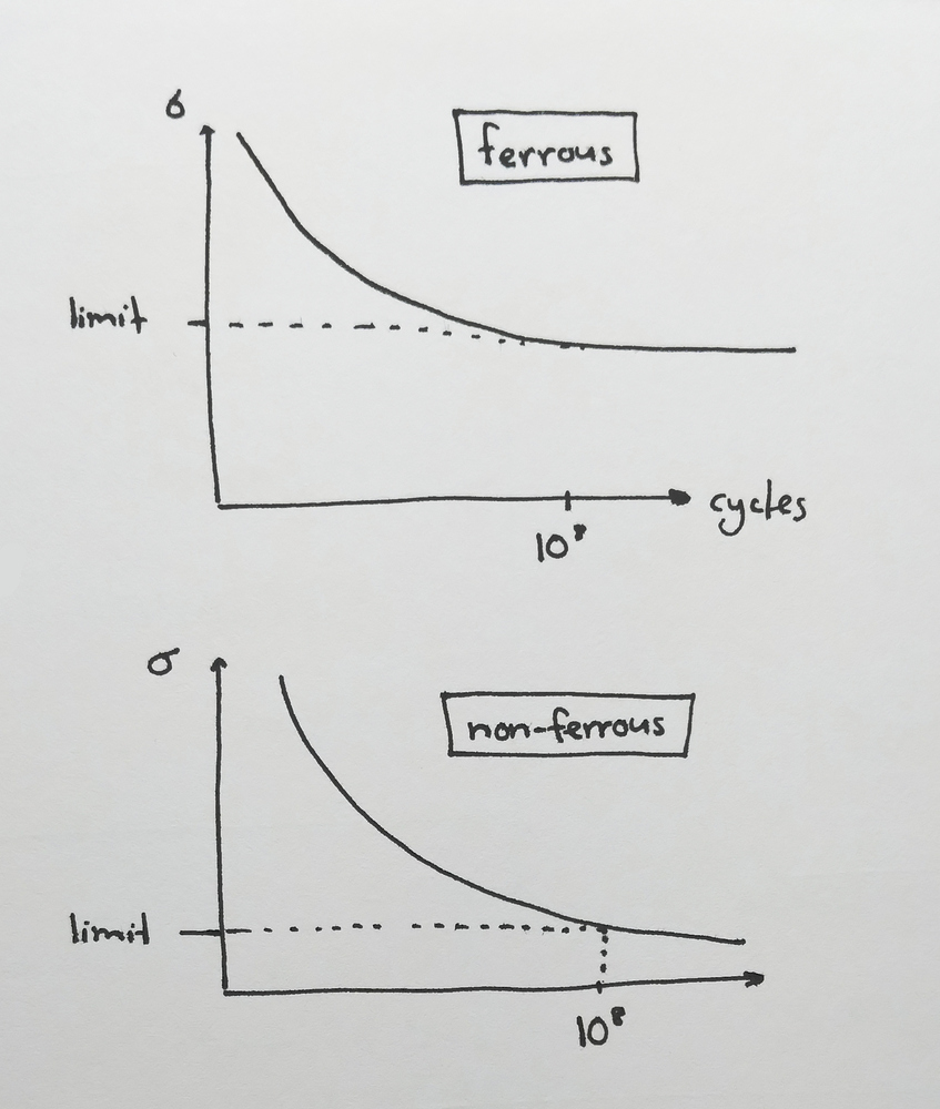
Stress (\sigma) is the amount of force being applied to an object per unit of cross-sectional area. If the cross-sectional area varies along the force axis, the smallest area is used. The unit of stress is \unit{Pa} (\N\m^{-2}).
Strain (\epsilon) is the amount of deformation in a material, expressed as the relative change in length (absolute change in length \Delta L over the original length L_0). It is dimensionless.
Elastic deformation is a temporary change to the shape of a material due to applied stress. The material returns to its original shape once the stress is removed.
Plastic deformation is a permanent change to the shape of a material. The material does not return to its original shape after the stress is removed. The amount of stress required before plastic deformation occurs is called the yield stress, yield strength, or \sigma_y. The yield stress of titanium is 820\unit{GPa} and of aluminium is 240\unit{MPa}.
Poisson’s ratio \nu is a measure of how much deformation a material experiences perpendicular to the applied force (transverse deformation) when stretched or compressed (axial deformation). The \nu of most metals is around 0.3, and of most polymers is around 0.5.
The strength of a material is the amount of stress it can withstand before some limit is reached.
Yield strength is the amount of stress a material can withstand before it experiences plastic deformation. This is equal to the stress at the yield point. For most metals a precise yield point cannot be determined, so the 0.2% proof stress is used instead (found by tracing a line upwards from the 0.2% strain point with gradient E).
Ultimate tensile strength (UTS) is the amount of stress a material can withstand before fracturing. This is equal to the stress at the apex of a stress-strain graph. In a brittle material, this is also equal to the yield strength, because brittle materials will fracture instead of plastically deforming.
The toughness of a material is the total amount of energy (work) per unit volume that it can dissipate/absorb before fracturing. Toughness is given by the total area underneath a stress-strain graph between the origin and the fracture point, and is measured in joules.
Ductility is the amount of plastic deformation that occurs in a material before fracturing, measured as either percentage elongation or percentage reduction in area. Ductile materials tend to be tough, but not strong, and will form a ‘cup and cone’ shape when fractured.
A material is brittle if it experiences no plastic deformation before fracture. The resultant fragments can be collected and slotted back together without any gaps. Examples of brittle materials are ceramics and glass. Brittle materials tend to be strong, but not tough.
Fracture is the point where one piece of material becomes many. A gap is often formed in the material at the point of fracture due to sudden recovery of elastic deformation.
Hardness is the resistance of a material to localised plastic deformation.
The indentation test is used to determine the hardness of a material. To perform the test, an indenter of a harder material than the one being tested is pressed into the material using a known force, and then the indentation created is measured. The smaller the indent, the harder the material.
Hardness is related to strength because the material must be plastically deformed in order to leave an indentation, and plastic deformation can only be performed by exceeding the yield strength of the material. Hardness is usually proportional to strength for isotropic materials (properties are uniform in all directions).
There are many different Rockwell scales used for hardness testing, using different indenters and different loads. Each scale measures from 0 to 100. Measured values can’t be compared across scales. Geologists use the Moh’s scale instead, which measures from 1 to 10.
Stress is tightly related to strain. A stress-strain graph plots the amount of strain experienced by a material as an increasing tensile stress is applied, with stress on the vertical axis and strain on the horizontal.
The initial strain in a material is due to elastic deformation. This elastic portion of the graph is a straight line, with the Young’s modulus E of the material being the gradient of this line (measured in Pascals). A steep slope indicates a stiffer material (steel, glass), and a shallow slope indicates a more elastic material (polyethylene). The Young’s modulus of titanium is 100\unit{GPa}, and of aluminium is 70\unit{GPa}.
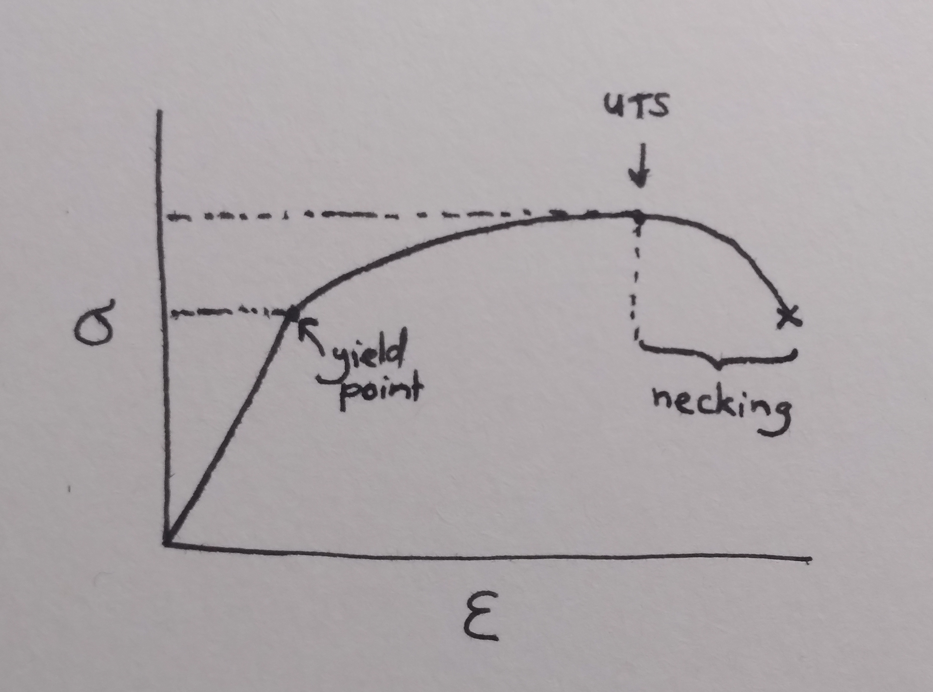
The yield point of a material is represented by a change in the gradient of the stress-strain graph. This is the point where the material stops undergoing further elastic deformation and begins to undergo plastic deformation. The stress at this point is called the yield stress (\sigma_y). If a precise yield point cannot be determined, the 0.2% proof stress is used instead (found by tracing a line upwards from the 0.2% strain point with gradient E).
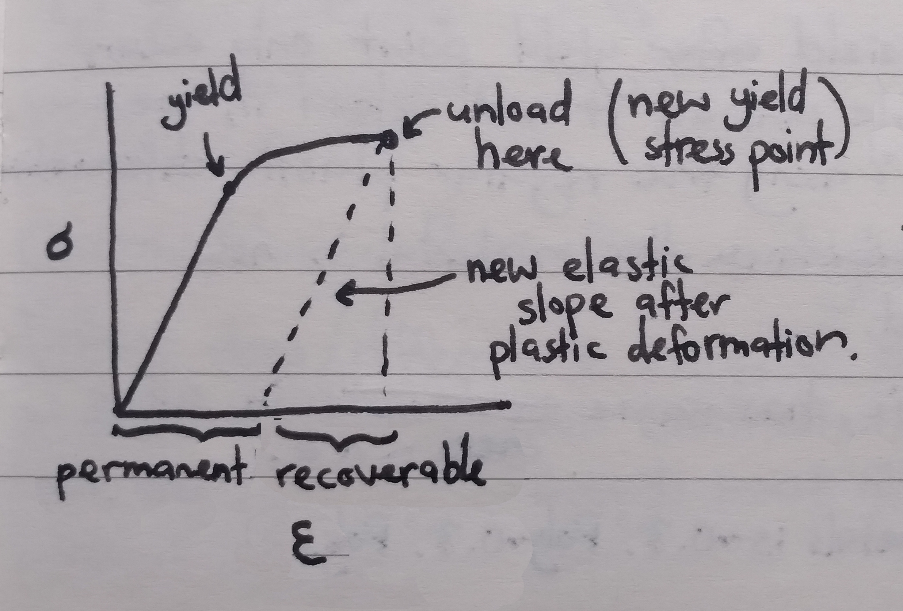
Continuing to strain the material past the yield point will ‘work harden’ the material (yield strength of a material increases with plastic deformation). If stress is removed after this point, the graph will descend with gradient E as the elastic portion of deformation is recovered. The point at which stress was removed is the new yield point of the material, and the distance between the original L_0 and the new length at rest measures permanent deformation. The curve will continue along the original trajectory once stress is reapplied.
Discontinuous yield is a phenomenon where the curve directly following the yield point is generally flattish with a lot of random noise. After this point the curve will become smooth again, even after the material is unloaded and reloaded. We’re told that this is (somewhat) unique to mild steel.
The stress at the peak of the curve is called the ultimate tensile stress, or UTS. Necking (localised reduction in cross-sectional area) occurs past this point up until fracture. This explains the downwards slope past the UTS, where the reduction in cross-sectional area leads to an increase in strain (due to the Poisson effect).
Since the stress on the graph is taken from the original cross-sectional area (engineering stress) there appears to be a reduction in stress after UTS, when in reality the reduction in cross-sectional area and continued increase in force would lead to an increase in stress.
Stress-strain curves show engineering stress, calculated from the original cross-sectional area of the material. In contrast, true stress is calculated from the real cross-sectional area (which changes continuously during the test). The engineering stress-strain curve starts to descend after the UTS, indicating the point where the cross-sectional area starts to reduce (necking).
Engineering stress is used because it’s simpler to calculate, and because engineering projects will never come close to exceeding the yield stress of a material anyway (as this would permanently damage the material, impacting the integrity of the project).
Crystallinity refers to the degree of long-range structural order in the atoms of a material. A crystal lattice structure has atoms arranged in regular repeating patterns. Solid metals tend to be crystalline solids.
We can represent a crystal lattice using a unit cell, the smallest tileable portion of the lattice.
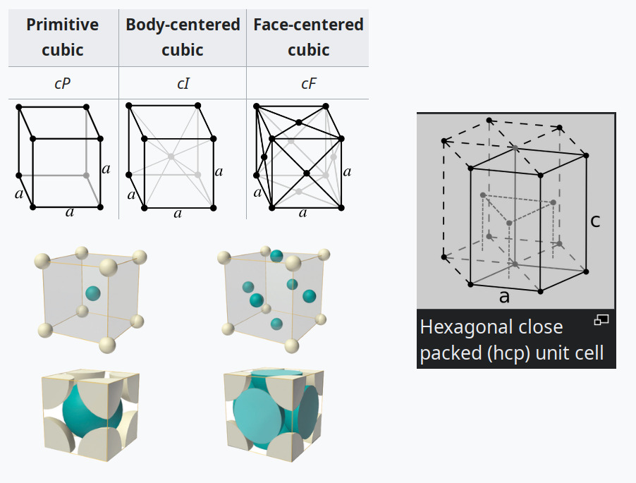
The three most common unit cells for metals are the body-centered cubic (BCC), face-centered cubic (FCC), and hexagonal close packed (HCP). FCC and HCP are close-packed structures, because they have the greatest possible atomic packing factor.
Polymorphic materials can exist in more than one structure. Iron is BCC at room temperature, but FCC at temperatures exceeding 912°C.
BCC
FCC
HCP
Atoms per cell
2
4
6
Coordination number
8
12
12
Unit cell dimensions
\frac{4R}{\sqrt{3}}
\frac{4R}{\sqrt{2}}
--
Atomic packing factor
68%
74%
74%
Examples
Cr, Mo, Fe
Cu, Al, Au
Mg, Ti, Zn
Physical properties
Brittle
Ductile
Very brittle
Atoms per cell The (fractional) number of atoms contained in the cell.
Coordination number the number of atoms bonded to any given atom in the lattice.
Unit cell dimensions Edge length a of the unit cell relative to the radius R of the atoms. To calculate, choose a close-packed vector in the cell, count the number of radii along that edge and divide by the edge length (a\sqrt{2} for a planar diagonal, a\sqrt{3} for a cubic diagonal).
Atomic packing factor The spherical packing ratio, given by the total atom volume over the cell volume, or atoms per cell times \frac{4}{3}\pi R^3 over a^3.
Ceramics are crystalline solids consisting of both metallic and non-metallic atoms and joined by a combination of ionic and covalent bonds. The crystalline structure is determined by the balance of charges (the resulting solid is electrically neutral) and by the relative sizes of ions (cations are positive and small, anions are negative and large). Cations can only bond with anions.
The two crystalline structures we’re looking at for ceramics are the rock salt structure (used by MgO, FeO, NaCl) and the silicate structure (used by rock, soil, clay, sand).
In the rock salt structure, each of the two atoms forms a separate face-centered cubic lattice, with the two lattices inter-penetrating to form a three-dimensional checker pattern. The interstitial sites of one lattice are filled with the atoms of the other. Coordination number is 6 (each cation only touches six anions, along cardinal directions), unit cell dimension in a = 2(R_a + R_c). Materials are thermally and electrically insulating, we’re told that this is due to a lack of free electrons.
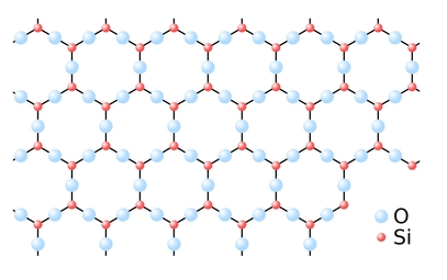
The silicate structure is based on the \ce{SiO4^4-} tetrahedra (\ce{Si} cation is +4, \ce{O} anions are -2). \ce{SiO4^4-} is not stable, but multiple of them can link together into a crystal lattice and sharing oxygen atoms (called ‘bridging oxygens’) to create \ce{SiO2} (silicon dioxide / silica), which has a neutral charge. Examples are quartz and amethyst (quartz with iron impurities).
Glass is an example of an amorphous silicate. Whether a silicate structure becomes crystalline or glass depends on how fast it cools from the liquid state. Rapid cooling doesn’t give the atoms time to arrange into a stable lattice, and so creates glass. The following image is a slow-cooled silicon dioxide (\ce{SiO_2}) crystal lattice.
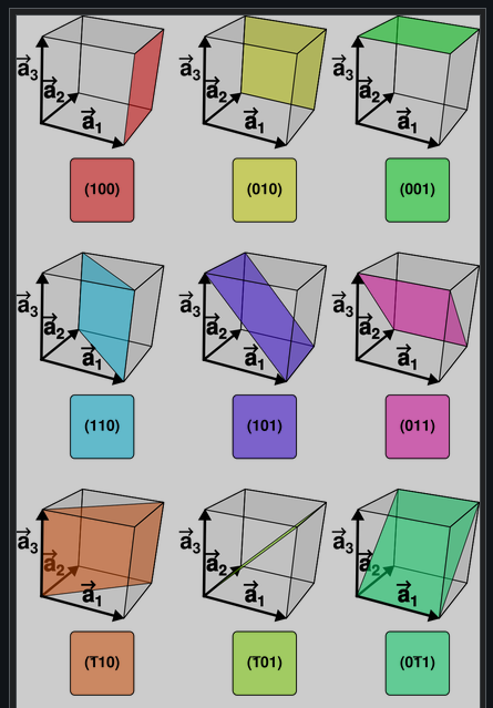
Miller indices describe how a plane intersects a unit cell. Each index is the reciprocal of the distance along a given axis, measured from the origin to the point where the plane intersects that axis. An index of 0 means that the plane runs parallel to that axis, 1 means that the intersection is at the far edge of the cell, and 2 means that the intersection is halfway along the cell (and also at the far edge). Planes repeat on a period of 1, so a negative index has the effect of reflecting the plane left-to-right along that axis (across the plane which bisects that axis in the cell).
Planes are denoted (h\ k\ l). Families of planes are denoted \{h\ k\ l\}, containing all planes which can be transformed into (h\ k\ l) by a symmetry operation that would leave the crystal unchanged (the planes are called ‘crystallographically equivalent’). Since we’re working with cubic cells, this includes any combination of reflections in all three axial planes. Specifically, for a cubic crystal, we just need to find all permutations of the three indices, including a positive and negative version of each index. The family \{1\ 1\ 0\} includes the 12 planes \{\pm 1, \pm 1, 0\}, \{\pm 1, 0, \pm 1\}, \{0, \pm 1, \pm 1\}. For lattices with lower symmetry, the planes in the family would be more constrained.
A similar notation is used for describing a ‘direction’ inside a unit cell (essentially a vector). Each index gives the distance along an axis from an origin where the direction intersects with the bounds of the cell, where 0 means that the direction is perpendicular to that axis. Indices are conventionally scaled to be integers (in other words, such that the greatest common divisor is 1), so the direction [1\ 0\ \frac{1}{2}] would become [2\ 0\ 1].
Directions within a cell are denoted [u\ v\ w]. Families of directions are denoted ⟨u\ v\ w⟩, containing all crystallographically equivalent directions in the same way as for planes.
Negative indices are denoted with an overbar, as in \{\bar{1}\ 0\ 1\}.
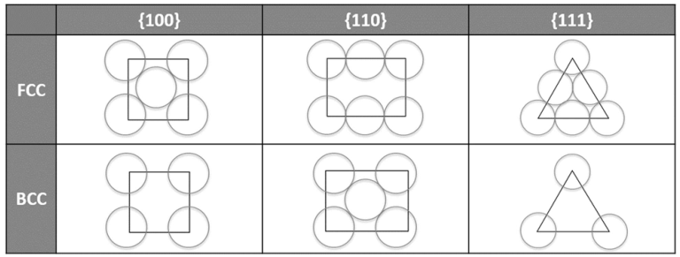
We can draw how a plane intersects with a unit cell in order to see how closely-packed the cell is along that plane. Only draw atoms where the center lies on that plane. The close-packed directions within that plane are those where the atoms are touching all along the line. A close-packed plane is one where all directions are close-packed, or in other words, where there is no gap between adjacent atoms.
If the atomic arrangement is the same on multiple planes, those planes are crystallographically equivalent.
In FCC, \{1\ 0\ 0\} is close-packed in ⟨1\ 1\ 0⟩ directions. In BCC, \{1\ 1\ 0\} is most closely packed in ⟨1\ 1\ 1⟩ directions, but doesn’t have a true close-packed plane.
During elastic deformation, the bonds between atoms stretch without breaking. This is analogous to spring deformation. The Young’s modulus E is an innate property of the material.
During plastic deformation, the bonds between atoms break and the planes in the lattice slide across one another, settling and re-bonding at the next closest stable position (this is easier in metals because there are a lot of free electrons). This is called slip. The model of slip that we use in this course is called box slip, where we look at unit cells in the lattice as cubes in a grid. In order for block slip to occur, every atom on the plane has to break and slip simultaneously, which requires a lot of energy.
On a close-packed plane, the distance to the next stable position is small, so the amount of energy/work (and therefore force) required to slip is small. This results in a weaker, more ductile material along that plane. In comparison, non-close-packed planes result in stronger, more brittle materials along that plane. This means that FCC materials tend to be more ductile, and BCC materials tend to be more brittle. An HCP structure has all close-packed planes lying in one orientation, so HCP materials are very strong and brittle (slip is very difficult).
The main slip system of a lattice is the planes and directions in which slip (and therefore deformation) can most easily occur (these are the closest-packed planes and directions).
The main slip system of an FCC lattice is \{1\ 1\ 1\}\ ⟨1\ 1\ 0⟩.
The main slip system of a BCC lattice is \{1\ 1\ 0\}\ ⟨1\ 1\ 1⟩.
For rock-salt structures, plastic deformation will cause cations to move to be adjacent to other cations, causing planes to repulse one another and the material to fracture. Plastic deformation of this structure is improbable.
The theoretical shear strength of pure elemental iron (based on the energy required to break bonds) is 10,000\unit{MPa}, but in practice the strength is only around 20\unit{MPa}. This is due to defects in the material.
One dimensional defects / point defects:
Vacancies An atom is missing from the crystal lattice, leaving an unfilled gap.
Substitutional atoms An atom is replaced with an atom of a different element in the lattice.
Interstitial atoms A smaller atom of another element is jammed into the interstitial space of a lattice.
Two dimensional defects / planar defects:
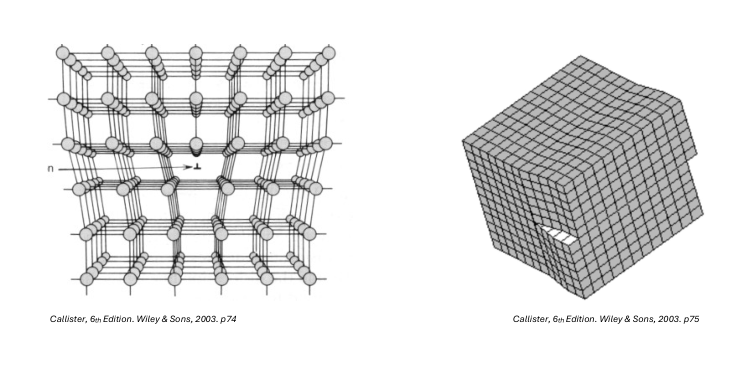
Edge dislocation An extra half-plane is inserted into the lattice.
Screw dislocation The lattice splits and twists such that the top and bottom interfaces of the split no longer align.
Dislocations in a lattice (notated as \perp) reduce the amount of energy required to slip because the plane can now slide one atom at a time, so fewer bonds need to break before slip can occur. Less work is required to slip, corresponding directly to a lower yield strength for the material. Slip happens most easily on close-packed planes in close-packed directions.
Dislocations cannot occur in ceramics due to the strict structure enforced by bonds between cations and anions.
Resistivity \rho is a property that affects how easily electrons can move through a material. The resistivity of a material depends on its crystal structure.
\rho = \frac{R \x A}{l}
Conductivity \sigma is the reciprocal of resistivity. It shares the same symbol as stress, which is a little confusing.
\sigma = \1{\rho}
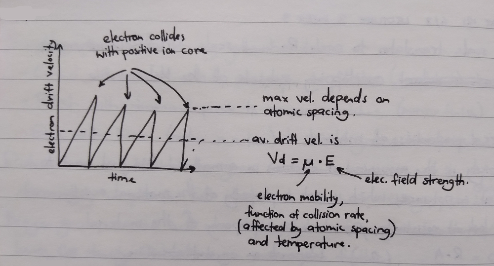
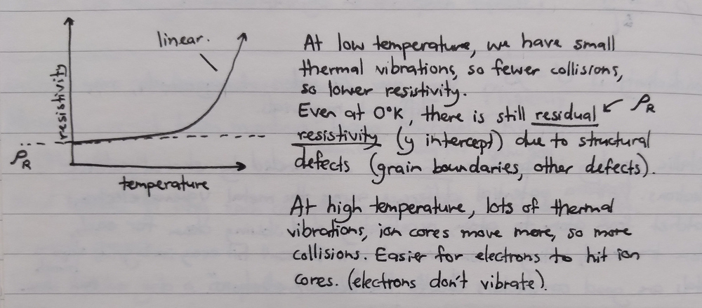
Metallic crystal lattices are formed from a lattice of positive ion cores surrounded by a cloud of de-localised electrons that can move freely through the lattice. When a potential difference is placed across the lattice, these free valence electrons ratchet from ion core to ion core, moving constantly towards the higher potential. As these electrons travel, they accelerate and then collide with the next ion core, increasing in velocity only to crash into the core and become stationary again (losing energy and generating heat). The electrons don’t hit every ion core along the path: if the temperature of the material is lower, the ion cores will vibrate slower, and there will be less chance that a given ion core will jump into the travel path.
The velocity of an electron moving through a metallic lattice can be modelled as a saw-wave graph, mapping electron drift velocity to time. Peaks on the graph indicate maximum electron velocity. Average drift velocity V_d is given by electron mobility \mu (a function of collision rate, affected by atomic spacing and temperature) and electric field strength E:
V_d = \mu \x E
Resistivity is non-linear with temperature.
\rho_T = \rho_{0°C} (1 + \alpha_T \x T)
The resistivity of metals increases (possibly linearly) as the percentage of cold work increases (as this increases the number of dislocations in the material).
Ceramics and glasses are very good insulators. There is no ‘sea of electrons’, all electrons in the lattice are tied up in covalent and ionic bonds.
Most metals are crystalline, but instead of being formed from a single coherent lattice (monocrystalline), they tend to be formed from many smaller interlocking lattices of different orientations (polycrystalline). These individual lattices are called grains. Grains that are roughly spherical in shape are ‘equiax’, and grains that are longer and narrower are ‘elongated’.
Metallography is the process of grinding, polishing, and etching a polycrystalline sample in order to reveal the grain structure. The process is as follows:
Slice a thin sample of the material, embedding it into a lump of epoxy resin for easy handling.
Grind with silicon carbide sandpaper to flatten the surface (creating a scratched surface)
Polish with diamond paste to remove scratches (creating a mirror finish)
Etch with an acid or alkali to selectively corrode grain boundaries (we used 3% Nital, nitric acid in ethanol). This corrodes the grain boundaries with a redox reaction, reducing their reflectance.
The individual grains can now be distinguished under a microscope.
Grains form when a metal is cooled from a molten state (amorphous, atoms moving freely past one another) to a solid state (atoms lock in place). As the metal begins to cool, some atoms cling to one another to form nuclei crystals, and as the metal cools further these crystals attract more atoms towards themselves, eventually forming a voronoi pattern of grains.
Grain nucleation falls into two categories. Homogeneous nucleation is where atoms cling spontaneously to one another in the molten material, forming the basis for a spherical grain. This is very rare. Heterogeneous nucleation is where atoms nucleate on a surface (called a mould), creating a flat grain spread across the surface, or nucleate on an atom of a different element. This is far more common (we’re told it has something to do with thermodynamics).
Grain boundaries are a form of imperfection. Atoms inside a grain are called bulk atoms, and atoms at a grain boundary are called surface atoms. All of the bonds of a bulk atom are fully formed (linked into the lattice on all sides), but a surface atom has ‘free’ bonds. This makes a grain boundary a high-energy region due to these free atomic bonds, which are then able to bond with other atoms to reach a lower energy state.
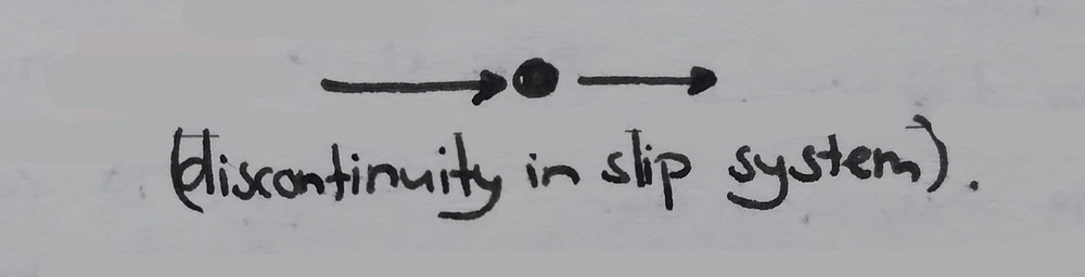
Grain boundaries inhibit the movement of dislocations because the lattices on each side of the boundary are discontinuous (‘discontinuity in planes’), breaking up any slip systems. Materials with many smaller grains are strong and brittle (‘higher grain boundary density’), and materials with fewer larger grains are weak and ductile (dislocations can move much further).
The Hall-Petch equation describes the relation between grain size and the yield strength of a material (I think it only applies to materials with equiax grains). \sigma_0 is the friction stress, the minimum stress required for dislocation movement to occur (or resistance of the lattice to dislocation motion), k is the strengthening coefficient or Hall-Petch constant, and d is the average grain diameter in millimetres. \sigma_0 and k are specific to each material.
\sigma_y = \sigma_0 + \frac{k}{\sqrt{d}}
When graphed, the x axis is \frac{1}{\sqrt{d}} (ranging from 0 to 0.3, smaller grains to the right), and the y axis is \sigma_y, with \sigma_0 being the y intercept. The gradient of the line is k and is positive. If we get smaller grains, we get an increase in yield stress.
Grains don’t form consistently through a material as it cools from molten to solid, because of the higher incidence of heterogeneous over homogeneous nucleation, and because the container that molten metal is poured into tends to be cooler than the metal itself. This means that most grains will form initially at the interface between the molten metal and the container.
An example used in class was the cross-section of a cast aluminium cylinder. To prepare the sample, molten 99.5% aluminium at 720°C (60°C above melting point) was poured into a mould made of 1” steel plate at room temperature and left to cool.
Initially, small equiax grains started to form on the mould walls due to heterogeneous nucleation (these grains are called chill crystals).
Next, columnar grains extended from the equiax grains, pointing towards the center of the mould.
Finally, larger equiax grains formed in the center of the sample, occupying roughly 50% of the cross-sectional surface area.
The aluminium contracted as it cooled, creating a large depression in what was the top surface.
There are multiple situations that can occur after the formation of columnar grains along the sample edges:
Equiax grains form in the center, bounded by the walls of columnar grains (most desirable outcome)
The walls of columnar grains keep extending until they meet in the center
Holes or pores form in the center (least desirable outcome)
Dendrites (columnar grains branch into tree structures) are formed
All of these situations are still non-optimal because the columnar grains make for an anisotropic material (a material that has different behaviour along different planes). What we most want is an isotropic material, one consisting entirely of equiax grains. This can be achieved by annealing the metal (heating then controlled cooling) or by using grain refiners (sprinkling Ti or Cd into Al to act as nucleation sites).
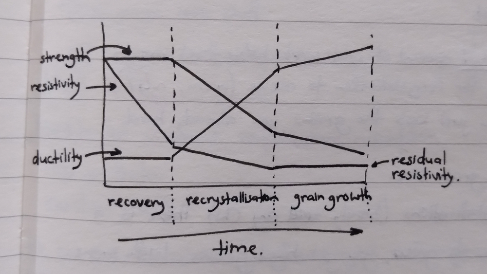
Annealing is a heat treatment that completely regenerates grains which have been deformed by cold work. This is useful for copper wiring for example, which is made brittle and resistive by the drawing process. Annealing transforms the strained longitudinal grains back into relaxed equiax grains, restoring ductility and conductivity. Annealing is generally performed at two-thirds of the melting point of the metal.
There are three stages to the annealing process:
Recovery Dislocations rearrange into a lower energy configuration, spreading out more evenly. Grains stay the same shape, the number of dislocations in the material stays the same, but the material does soften a little.
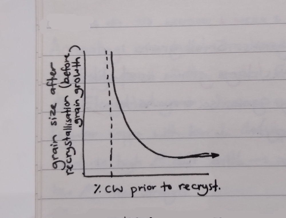
Recrystallisation New grains nucleate at grain boundaries (which are high energy sites) by consuming stored strain energy. These nuclei will then increase in size by cannibalising atoms from the neighbouring elongated grains, eventually replacing those grains completely with new equiaxed grains with low dislocation density / internal stress. If the material hasn’t been sufficiently cold-worked prior to annealing (called the ‘critical cold work’, normally around 4\%), then there won’t be enough stored strain energy to nucleate these new grains and kick off the recrystallisation process. The more cold work is performed prior to annealing, the greater the number of grains that will be able to nucleate, and the more and smaller the resultant equiaxed grains will be (because there will be less room to grow). The material will also be stronger as per Hall-Petch.
Grain growth If the material is kept hot following complete recrystallisation, the grains will continue to grow and cannibalise each other to a point, resulting in a coarser grain structure (fewer grain boundaries is a lower-energy state).
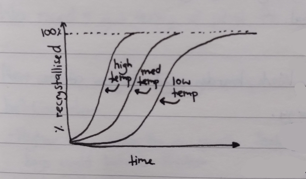
The recrystallisation temperature of a material is the temperature at which a 50\% cold-worked sample will fully recrystallise in exactly one hour. If the percentage of cold work is lower, the recrystallisation temperature will be higher to make up for the energy deficit, and vice versa. This is an intrinsic property of the material. The table below is given in °C.
Metal
Melt
Recrys.
Lead
327
-4
Aluminium
660
80
Copper
1085
120
Iron
1538
370
When a material is hot-worked (worked above the recrystallisation temperature), it will continuously recrystallise while you work-harden it.
When a polycrystalline material is plastically deformed, the individual grains will also become deformed. Running a material through rollers will flatten equiax grains into elongated grains. The grain volumes do not change.
When dislocations start slipping, we get also get multiplication of dislocations. Dislocations initially allow materials to slip easier, but each movement significantly increases the number of dislocations in the material and this acts to prevent the movement of other dislocations (because dislocations are planar discontinuities). The strength of the material increases until it loses the requisite ductility and the material fractures. There are also diminishing returns when using cold work to increase the hardness of a material — once the material is saturated with dislocations, adding more won’t meaningfully increase the hardness.
Cold work is where a material is plastically deformed at a temperature below its recrystallisation temperature. The amount of cold work experienced is given as a percentage (‘percentage of cold work’). This can be measured either as a change in thickness (when rolling a material) or a change in cross-sectional area (when drawing a material). t_0 is the original thickness, t_f is the final thickness, and then the equivalent for cross-sectional area. These equations rely on the assumption that the width of the material doesn’t change much.
Atoms move within a solid crystal lattice via solid state diffusion (as opposed to liquid state diffusion). Solid state diffusion can be by vacancy diffusion, where a vacant site moves across a lattice, or by interstitial diffusion, where small atoms move through interstitial spaces in the lattice (there might be other forms too). Diffusion is modelled as a random walk.
Solid-state diffusion is prevented by an energy barrier Q (called the activation energy), which is normally provided in the form of heat. The atom (or vacancy) will then move to the next stable position in the lattice. Solid-state diffusion is normally really, really slow, but increases exponentially with heat.
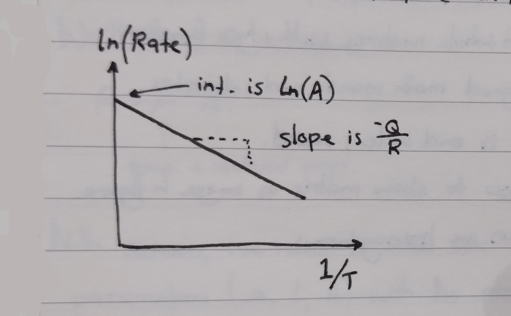
The Arrhenius equation models the diffusion coefficient D (rate of diffusion, given in \m^2/\s) given by a constant D_0, the activation energy Q (in \unit{J}/\unit{mol}), the gas constant R (8.314 \unit{J}/\unit{mol}\x\unit{K}), and the absolute temperature T (in kelvins).
D = D_0 \exp \left( \frac{-Q}{RT} \right)
This is plotted with \frac{1}{T} on the x-axis and with \ln(D) on the y-axis. This is because D increases exponentially as the reciprocal of temperature increases, so plotting in this way gives a straight line graph where the y-intercept is \ln(D_0) and the slope is \frac{-Q}{R}.
When salt is dissolved in water, we get a phase change. The water breaks the ionic bonds in the salt, creating a one-phase solution of salt (the solute) in water (the solvent). The salt solution saturates past a certain point, meaning that the water cannot dissolve any more salt, and you get salt precipitating on the bottom (a second phase, solid).
A phase is a “component within a system that has uniform physical characteristics”. The boundary between two phases is a phase boundary.
A solid is able to dissolve in another solid via solid-state diffusion. If both solids are metals, we call the resultant solution an alloy. An interstitial solid solution results from having tiny atoms dissolve in a matrix of larger atoms (such as carbon in steel). A substitutional solid solution results from having atoms replace other atoms of a similar size in a matrix (such as nickel in copper).
Solid solubility can be limited, where the parent matrix can only accept a certain percentage of solute before it saturates, or unlimited, where any proportion of either metal is possible. Interstitial solid solubility is always limited (C-Fe), substitutional solid solubility can be either limited (Cu-Ag) or unlimited (Cu-Ni).
A phase diagram shows which phases exist at equilibrium for various compositions and temperatures of a binary alloy. A material is at equilibrium when the temperature is constant throughout the material and is only increasing or decreasing very slowly.
We can use the lever rule to find the percentages of each phase that exist in an alloy system at a given composition and temperature:
Draw a point at the given composition and temperature.
Extend a line horizontally to the left and to the right until each end hits a phase boundary. These phase boundaries will border regions of pure phase.
To find the proportion of the mixture that is in a given phase, take the length of the line on the opposite side of that phase over the full length of the line. For example, if the phase boundary on the left is the liquidus (marking the full melting point), take the length of the right-hand line segment (extending from the point to the solidus). This can be see intuitively by thinking of a situation where the point is almost at the liquidus, with 10% of the line extending to the liquidus and 90% extending to the solidus — we know that the mixture must be mostly liquid with very little solid, so the proportion of liquid is 90%.
To find the composition of each phase, look at the percentage of solute that exists at that temperature at each end of the line. If the line intercepted the liquidus at 20% solute, then of the 90% liquid phase in the mixture, 20% is solute and 80% (100-20) is solvent. If the line on the other side intercepted the solidus at 40% solute, then of the 10% solid phase in the mixture, 40% is solute and 60% is solvent.
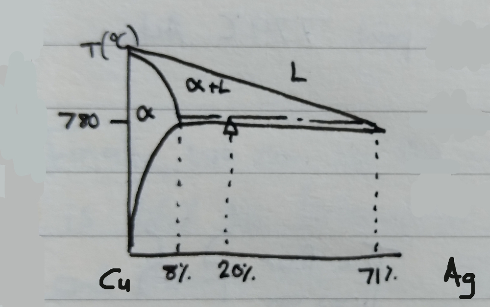
For example, if we have an Cu-Ag alloy at 780°C containing 20% Ag (as seen in the following phase diagram):
We measure a line to the left of our point, hitting the \alpha solidus, and to the right, hitting the liquidus.
The amount of solid \alpha phase in our alloy at this point is \frac{71-20}{71-8} = 81\%, and the amount of liquid phase is \frac{20-8}{71-8} = 19\%.
Of the 81% solid \alpha state, 8% is Ag and 92% is Cu. Of the 19% liquid state, 71% is Ag and 29% is Cu.
Bringing it all together, we can see that 81\% \times 8\% + 19\% \times 71\% = 20\%, which is the amount of Ag we started with.
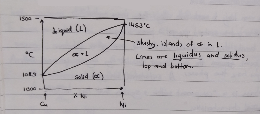
Binary isomorphous alloys are alloys of two elements with unlimited solid solubility. These alloys have two phases: a liquid phase, and a single solid phase \alpha. The atoms of the two metals are very similar in size — our example was Cu-Ni. The melting point of the alloy depends on the percentage of solute.
As the material cools, islands of solid \alpha form just below the liquidus, becoming big grains separated by small amounts of liquid just above the solidus, and then becoming a polycrystalline solid below the solidus.
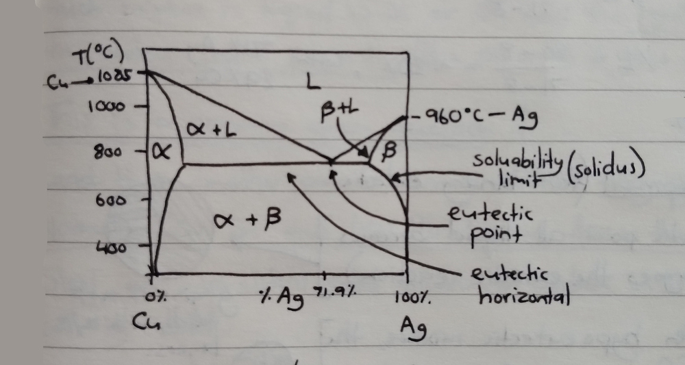
Binary eutectic alloys are alloys of two elements with limited solid solubility. These alloys have three phases: a liquid phase, a solid phase \alpha of majority one element, and a solid phase \beta of majority the other element. The atoms have a bit more of a size difference — our example was CuAg — such that only so much Ag (8%) can dissolve in Cu, and only so much Cu (8.8%) can dissolve in Ag. This solubility limit also changes with temperature.
Eutectic means ‘easily melted’. Binary eutectic alloys have a composition where cooling will transition directly from a liquid state to a solid state, with no intermediary ‘slushy state’ — this composition is called the eutectic composition (which depends on the alloy), and the exact transition point for this composition is called the eutectic point. The temperature that divides the liquid state from the solid states is called the eutectic temperature, or otherwise the eutectic horizontal.
When cooling below the eutectic temperature, the material undergoes the eutectic reaction, spontaneously forming finely interleaved layers of \alpha and \beta solid phases (a eutectic structure). This eutectic structure is very strong because of the very finely layered grain structure, which helps to block dislocation movement. The layers form through liquid-state diffusion.
The eutectic reaction occurs even if the mixture lies to the left (hypo-eutectic) or right (hyper-eutectic) of the eutectic point, because as the temperature cools towards the eutectic temperature, the excess Cu or Ag in the mixture sweat out into islands of pro-eutectic\alpha or \beta, leaving the liquid phase at exactly the eutectic composition by the time the mixture reaches the eutectic temperature.
The proportion of eutectic structure in a solid of a particular composition can only be calculated by looking at the phase percentages just above the eutectic temperature, because some of the \alpha or \beta in a a hypo- or hyper-eutectic composition will have gone towards pro-eutectic solid instead. The percentage of liquid state in the mixture will exactly equal the percentage of eutectic solid that will form.
If the composition instead causes the point to travel through the pure \alpha (or \beta) phases at either edge of the diagram, you’ll begin with 100% liquid phase, which cools into the pure \alpha region to become pure poly-crystalline \alpha. As it cools further, the solubility limit of the \alpha drops and the excess Ag sweats out to form new grains of \beta at grain boundaries.
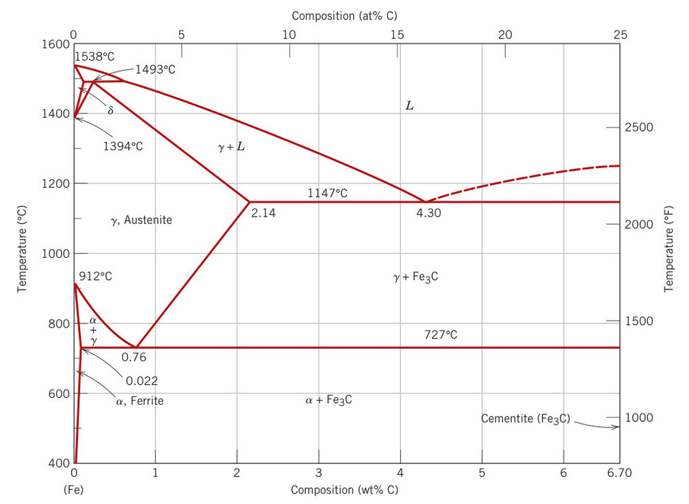
Steel is a very complex binary alloy (C-Fe). Carbon atoms are very small and can only slot into the interstitial spaces formed by the spherical packing of iron atoms. These interstitial spaces change dramatically when the iron lattice transitions from a BCC lattice to an FCC lattice above 723°C. The maximum solubility of C in Fe is 6.67%.
Steel can be categorised into ranges based on carbon content. Up to 0.25% C is called low carbon steel (also called mild steel), up to 0.5% C is called medium carbon steel, up to 0.95% C is called high carbon steel, and up to 4% C is called cast iron.
We care about three phases of steel:
\gamma — Austenite (gamma iron) FCC, holds up to 2.1% C. Exists above 723°C. Ductile, non-magnetic.
\alpha — Ferrite (alpha iron) BCC, holds up to 0.02% C. Magnetic.
\ce{Fe_3C} — Cementite (iron carbide) Ceramic, holds exactly 6.67% C. Very brittle (no slip systems).
Steel has both a eutectic temperature (at 1147°C) and a eutectoid temperature (at 727°C). The eutectoid temperature acts identically to the eutectic temperature from before.
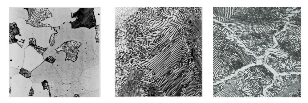
The eutectic structure of steel is called pearlite, which is formed from austenite (\gamma) of exactly 0.8% C composition. Pearlite is formed as interleaving thick layers of ferrite and thin layers of cementite. Unlike the eutectic structure, pearlite forms through solid-state diffusion, which is very slow, requiring very slow cooling. As before, we can have hypo- and hyper-eutectoid steels, and we can have chunks of pro-eutectoid \alpha or \ce{Fe_3C} in the mix forming at grain boundaries.
When eutectoid austenite (\gamma_{0.8}) is cooled slowly it forms coarse pearlite. The longer time spent at a higher temperature allows for greater solid-state diffusion, allowing the carbon atoms to move further and clump into thicker layers. When eutectoid austenite is cooled quickly it forms fine pearlite because the carbon atoms can’t move as far, forming closer layers. Fine pearlite is stronger and less ductile than coarse pearlite.
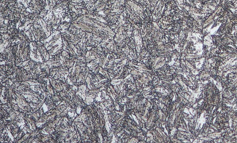
Cooling austenite rapidly through quenching creates martensite, a meta-stable phase of steel.
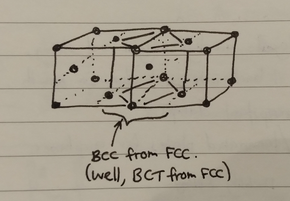
Normally, when austenite passes through the eutectoid temperature the iron lattice transitions from an FCC structure to BCC, with carbon solubility dropping from 2.1% to 0.02%. When quenching, however, there is no time for solid-state diffusion to occur, so the carbon atoms are trapped in place and the FCC structure changes instead to BCT (body-centered tetragonal, an elongated form of BCC). This is less of a change and more of a reinterpretation of the FCC structure (I don’t really understand this one). BCT has almost no slip systems and is extremely hard and brittle. The hardness of martensite increases with higher percentages of carbon (which creates lattice distortion, applying stress to the lattice).
Martensite is a highly unpredictable material due to how brittle it is. It can be made much more predictable through tempering (dispersion strengthening), which disperses fine \ce{Fe_3C} precipitates through the matrix. The martensite becomes \alpha + \ce{Fe_3C}, which is the same combination of phases as pearlite but with a very different structure. The BCT structure of martensite is only stable while carbon atoms are trapped inside it. When these carbon atoms diffuse out, the BCT \alpha_{ss} reverts to regular BCC \alpha. Tempered martensite has optimal strength with sufficient ductility for high toughness.
The properties of tempered martensite vary with the amount of time that the material is tempered for. As the material tempers, fine particulates will begin to clump (as per dispersion strengthening), leading to a more ductile material and less strong material.
Phase diagrams are only applicable when a material is at equilibrium, being heated or cooled extremely slowly. It can’t tell us what happens in a material as you heat or cool it more quickly.
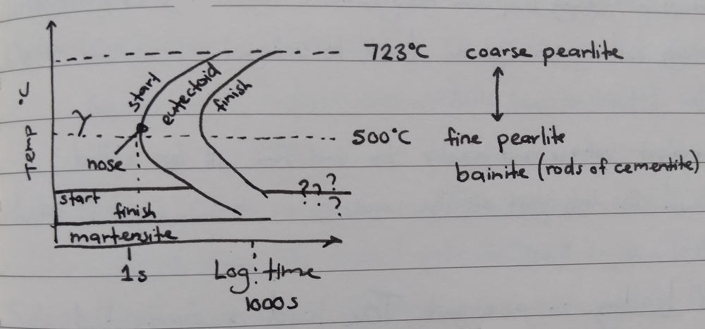
A TTT diagram allows us to see changes in a material of a fixed temperature over time (an isothermal transformation diagram). To use it correctly, you need to rapidly cool to a specific temperature and then hold there.
The swooping curve represents the zone at which pearlite is formed. The left-most point on the curve is called the nose, and it is at this point that fine pearlite is formed. At higher temperatures we get coarse pearlite, and at lower temperatures we get bainite, which is outside of the scope of this course. At much lower temperatures we get martensite. It takes about 1 second for pearlite to form; if we need more time, we can extend this out to about 20 minutes by alloying the steel with 1% Mg.
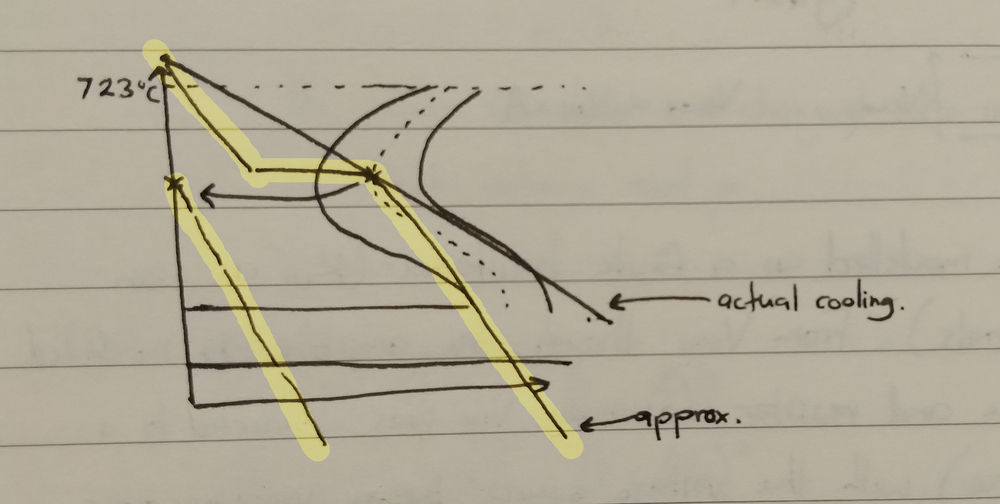
When continuous cooling is needed, a continuous cooling curve is used instead, but that’s outside of the scope of this course. We can, however, approximate continuous cooling with a TTT diagram.
We trace the actual temperature curve on the chart (seen below in yellow). In this example, we cool to around the nose point, forming fine pearlite. If we decide to continue cooling after the 50% pearlite mark, the composition of the material will be 50% pearlite and 50% austenite. We shift the cooling curve back to t=0 to see what happens with the austenite (the pearlite is already locked in), and we see that the curve plunges directly into the martensite zone without touching the eutectic curve, so we end up with 50% fine pearlite and 50% martensite.
Quenching steel can cause structural issues related to cooling speed. The surface of the steel cools much faster than the center, and as mentioned before the time taken for pearlite to begin to form is only 1 second, so a thick steel rod when quenched will become concentric layers of martensite, then bainite, and then fine and coarse pearlite.
As before, the addition of 1% Mg to the alloy will extend out this time period, allowing for a more consistent structure to form when quenched.
Spheroidising is a weakening mechanism. Slow-cooled high-carbon steels contain a lot of hard and brittle \ce{Fe_3C}, which wears out machining tools more quickly. To remedy this, the steel can be made temporarily soft and ductile while it’s being machined, and then heat-treated to make it hard again afterwards.
We can convert \ce{Fe_3C} layers in the steel into spheres by heating the material to around 700°C and holding it there for several hours, allowing for heavy diffusion of the carbon within the steel. These layers draw inwards, creating individual spheres dispersed throughout a ferrite matrix. A sphere has the highest volume to surface area ratio of any shape, so the surface area of \ce{Fe_3C} in the steel is reduced.
To revert the spheroidisation, the material is heated above the eutectoid temperature (forming austenite), and then cooled to form pearlite.
To strengthen any material, we’re really just looking to disrupt slip systems to inhibit dislocation movements, preventing plastic deformation.
For pure metals and alloys:
Cold work Multiply the density of dislocations in a material through cold work (dislocation movements are inhibited by dislocations, ‘traffic jam’).
Hall-Petch Increase grain boundary density through cold work and annealing, making grains smaller (dislocation movements are inhibited by grain boundaries).
For alloys:
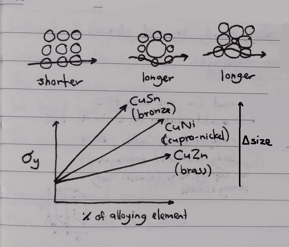
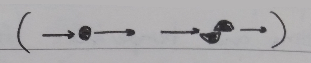
Lattice distortion Increase the equilibrium distance in the lattice by introducing atoms of much larger or smaller elements. These atoms have to stay in close contact with neighbouring atoms in the matrix, but the difference in sizes introduces distortion so that the path length through any one chain of atoms becomes longer.
Multiphase strengthening Increase phase boundary density through the eutectic/eutectoid reaction, creating fine layers of alternating phases (dislocation movements are inhibited by phase boundaries).
Dispersion strengthening Quench to form a super-saturated \alpha phase, then temper to finely disperse hard precipitates throughout the material (dislocation movements are inhibited by hard precipitates).
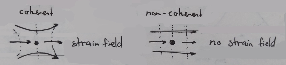
The larger the size difference between the atoms of the two elements, the greater the distortion of the lattice. The distance along each path / slip system in the lattice is increased by the distortion, which increases the equilibrium distance, which increases the yield strength of the material. Note that the atoms must be coherent with the matrix in order to distort the slip systems in this way.
Dislocations are stopped by phase boundaries, similarly to with grain boundaries, so we can strengthen a material by increasing the density of phase boundaries through the eutectic/eutectoid reaction.
The example given to us in class was in the use of AlCu alloys for aircraft fuselages. AlCu is a binary eutectic alloy with two solid phases:
\alpha, a solid solution of Cu in Al. Both Al and Cu are FCC, so \alpha is also FCC. Ductile.
\theta, the compound \ce{CuAl_2}. This is BCT / body-centered tetragonal, an elongated form of BCC, which has almost no slip systems. Extremely strong and brittle.
To effectively strengthen this alloy through multiphase strengthening, we want an alloy of the eutectic composition, maximising the amount of eutectic solid that forms on cooling. If we fall on either side of the eutectic composition, we’ll end up with clumps of pro-eutectic \alpha or \theta which will allow much more dislocation movement than eutectic structure alone. Pro-eutectic \theta is very strong and brittle, which makes for a very unpredictable material. Pro-eutectic \alpha is very weak and ductile. Eutectic structure itself is quite strong and a little ductile.
Dispersion strengthening works by distributing small precipitates through the metal (the parent matrix), which act to interrupt slip systems. This is also called age hardening or precipitation hardening.
There are some restrictions before we can perform dispersion strengthening:
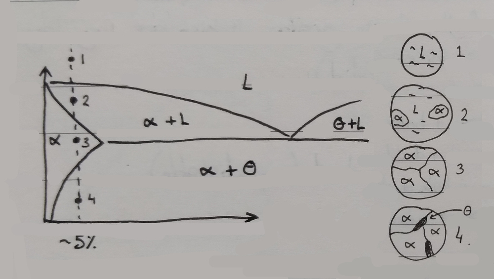
The phase diagram should exhibit decreasing solid solubility of the strengthening phase (\theta, the brittle phase) with decreasing temperature to allow super-saturation when quenching. This refers to the positive gradient of the \alpha boundary below the eutectic temperature on a binary eutectic phase diagram. An alloy where this isn’t the case is brass.
The parent matrix should be relatively soft and ductile to provide toughness, and the strengthening precipitate phase should be hard and brittle and finely dispersed to provide strength.
The alloy should be able to survive the quenching process (thermal shock will cause some materials to deform or fracture when quenched).
The precipitant should be:
hard and brittle, otherwise the precipitant will be sheared by applied forces
many and small, to better distribute through the material and lie in the way of any possible slip path (the center of a large precipitant is wasted, because dislocations are already stopped by the edges)
coherent with the parent matrix, in order to generate a strain field / lattice distortion, increasing the distance between equilibrium states and further increasing yield strength
Dispersion strengthening is performed according to the following process (for an example hypo-eutectic AlCu alloy):
The material is heated to a point above the solidus, such that it consists entirely of polycrystalline \alpha.
The material is cooled rapidly (quenched), passing into the \alpha + \theta region of the phase diagram. Normally, the reduction in solid solubility at this point would cause \theta to sweat out, forming brittle grains at grain boundaries. However, the rapid cooling doesn’t allow time for solid-state diffusion to occur, and the excess Cu is trapped inside the \alpha state. This creates a super-saturated \alpha state (written \alpha_{ss}), which is meta-stable and stronger than regular \alpha (due to excess Cu). The \alpha_{ss} is a very high energy state in a local minima, remaining stable until a nudge of energy gives it the ability to finally shed the excess Cu, returning to a much lower energy \alpha state.
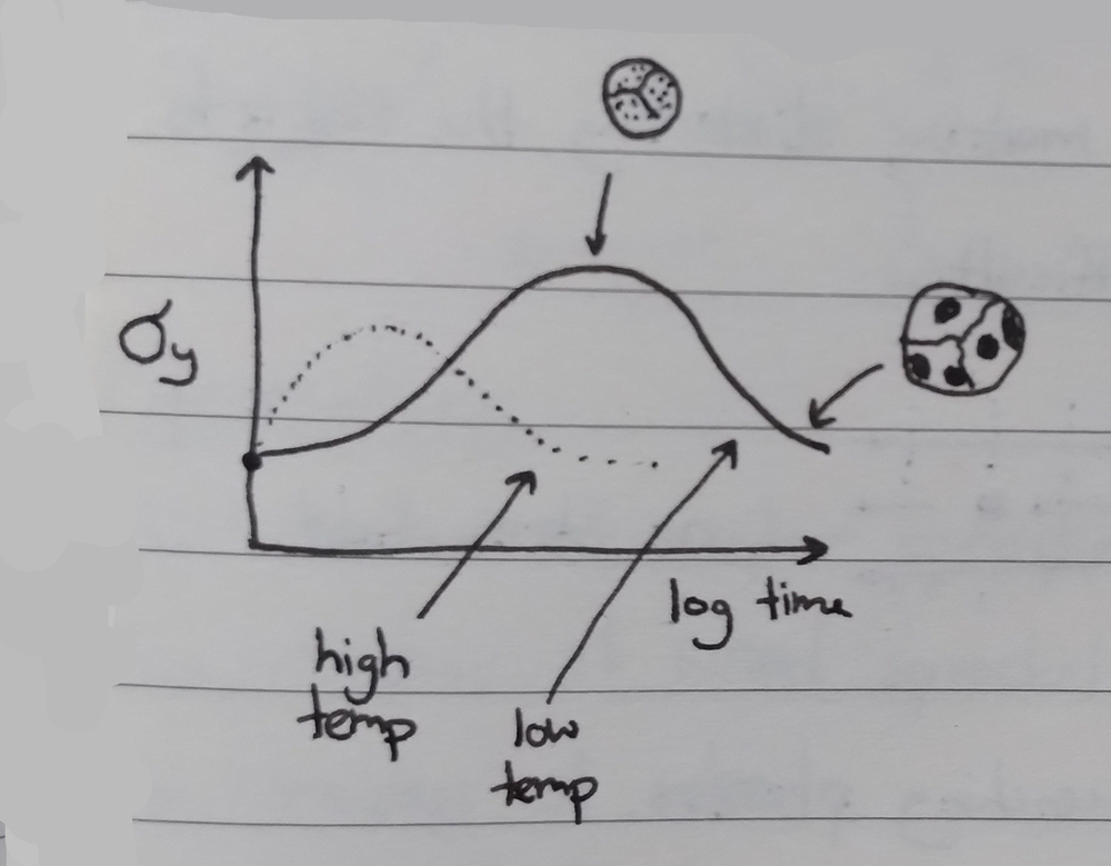
The material is heated to a point below the solidus to allow diffusion to finally occur. This would normally cause grain of \theta to form at grain boundaries (high-energy areas), but the \alpha_{ss} is much higher energy, so tiny grains of \theta form evenly throughout the material. This precipitation is caused by diffusion, and so is governed by time and temperature (as per the Arrhenius diffusion equation).
The lower the diffusion temperature, the smaller the precipitants and the stronger the resultant material. We want to use lower temperatures and longer times (3 hours vs 20 minutes) in order to obtain the strongest possible material. After too long, solid-state diffusion causes the \theta precipitants to start to clump, reducing strength again. Precipitation doesn’t end once the material reaches room temperature either, diffusion slows but does not stop. This means that older alloy samples have a tendency to be stronger than newer samples (unless they make it past the hump, I guess).
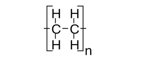
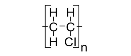
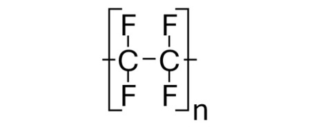
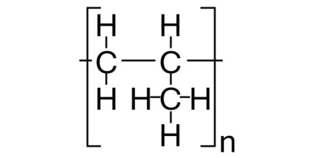
Organic chemistry is the study of carbon-based molecules, which tend to contain a backbone of carbon atoms with hydrogens (or other atoms) bonded at the edges.
Molecules are named after a set of basic rules:
A prefix of meth/eth/prop/but/pent/hex/... indicates the number of carbon atoms along the central chain (1, 2, 3, ...)
A suffix of -ane/-ene/-yne/... indicates the maximum number of bonds between any two carbon atoms (single, double, triple, ...)
An additional -ol suffix indicates the presence of an oxygen-hydrogen pair (an alcohol group).
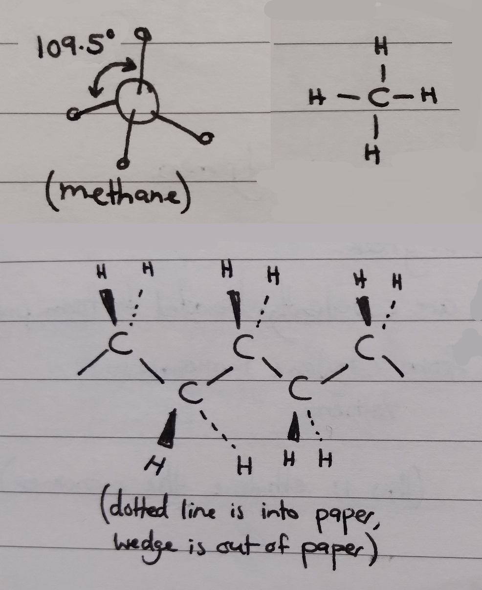
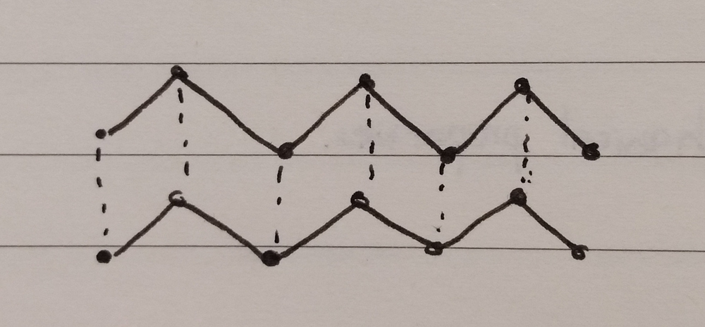
The simplest organic molecule is methane (\ce{CH_4}) which consists of a single carbon bonded to four hydrogens. Adding another carbon gives ethane, then propane, butane, etc. The angles between bonded hydrogens or carbons are a constant 109.5° due to Coulomb forces repelling adjacent atoms from each other. This angle causes the carbon-carbon backbone to form a permanent zig-zag shape, which makes polymer chains tangle and wrap around each other easily (bonds can rotate as long as the angle is preserved).
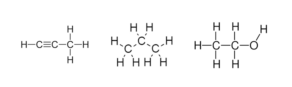
The molecules in the following picture are:
propyne (3 carbons, triple bond)
propane (3 carbons, single bond)
ethanol (2 carbons, single bond, with an oxygen-hydrogen pair)
Degree of polymerisation is a measure of the length of a polymer chain, as the number of monomer units making up the chain. Higher numbers represent longer chains, directly correlating with the mechanical properties of the material.
\text{DP} = \frac{\text{avg. molecular weight of polymer chains}}{\text{weight of a single monomer unit}}
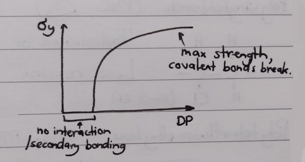
The degree of polymerisation directly correlates with yield strength:
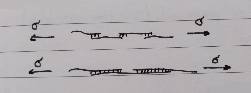
Polymers with a low degree of polymerisation (short chains) have few secondary bonds, which are easy to break or untangle (weak forces allow chains to slide against each another).
Polymers with a high degree of polymerisation (long chains) have lots of secondary bonds, making them very hard to break or untangle (high forces prevent chains from sliding against each other). Longer chains are also more likely to tangle in the first place.
With a sufficiently high applied force, the strength of the material comes entirely from the strength of the carbon-carbon backbone, not the intermolecular forces.
Polymer bulk structures range from amorphous to partially crystalline.
When amorphous, polymer chains are mixed together with no long-range order. Chains form a squiggly noodly mess with no mechanical strength. Amorphous structures are completely transparent, because the material is not dense enough to create internal reflections or refractions — light travels straight through.
When partially crystalline, sections of polymer chains zigzag against each other, forming long-range order. These regions with densely layered zigzags (crystallites) create lots of secondary bonds, and so have higher strength. Higher degrees of crystallinity (ranging from 5% to 95% crystallinity) correspond with higher strength and opacity and lower ductility. Opacity is caused when the crystallites become larger than the wavelengths of visible light, causing internal reflection and refraction.
Complete crystallinity is not possible, because the ‘folds’ in the crystallites are still random and the regions between crystallites are still amorphous.
If multiple chains lie in parallel to one another, we call the resultant structure a crystallite too (“ordered packing of multiple chains”).
Factors that affect the degree of crystallinity of a polymer are:
Rate of cooling Cooling a polymer slower allows polymer chains to form into folded crystallites structures. Rapid cooling causes the chains to freeze in place instantly, and because the material was hot, the structure will be amorphous.
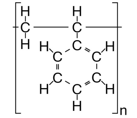
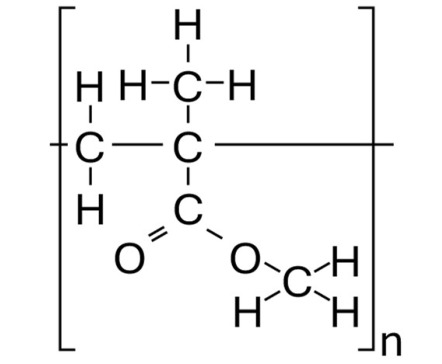
Presence of side groups Large side groups on a monomer (on PMMA, for example) will prevent the chains from folding tightly, leading to a less crystalline material.
Atactic side groups Atactic polymers have side groups distributed randomly along both sides of the polymer chain, preventing the chain from packing tightly (we’re given an example of a carbon backbone with scattered \ce{CH_3} methyl side groups). The amorphous chain leads to a low concentration of secondary bonds and poor mechanical properties.
Isotactic side groups Isotactic polymers have side groups distributed all along one side of the polymer chain. This creates lots of regular, repeating secondary bonds where the side groups are in contact with neighbouring chains, leading to a tightly packed, highly crystalline material with good mechanical properties.
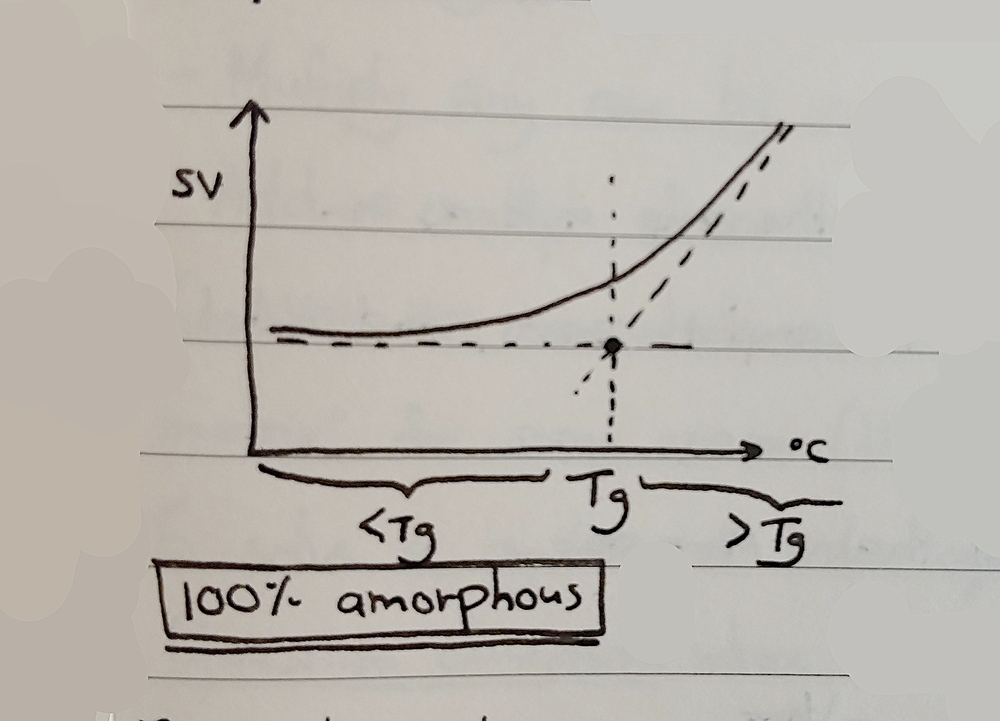
The glass-liquid transition is the gradual and reversible transition from a hard and brittle ‘glassy’ state to a viscous ‘rubbery’ state as temperature is increased. This can occur in amorphous materials, or in amorphous regions of semi-crystalline materials. The glass-transition temperature T_g is the temperature around which this transition occurs, which is difficult to measure exactly. The T_g of a material has consequences for performance at different temperatures, such as with rubber O-rings failing at colder temperatures.
Below T_g, the polymer is a glassy, brittle, amorphous solid. Individual polymer chains are locked in place and can’t slide, so the material is able to undergo elastic deformation.
Above T_g, thermal vibrations cause the polymer chains to start to slide against one another, causing the amorphous regions of the polymer to soften while crystalline regions remain stiff. The polymer is tough and leathery, but not brittle. If the polymer is completely amorphous, it becomes soft and moldable instead, becoming a viscous fluid with high enough temperature.
At T_m (the melting point), the secondary bonds are overcome by the thermal vibrations and the crystalline regions unravel into amorphous material with low viscosity. This unravelling is accompanied by a sudden increase in specific volume (SV, reciprocal of density). This can be seen visually by a decrease in opacity. Only crystalline or semi-crystalline polymers have a melting point.
When graphing temperature versus specific volume, more crystalline polymers will experience a sudden increase in specific volume at T_m, whereas more amorphous polymers will experience a gradual increase through T_g and T_m. This is because the melting point of a polymer is where crystallites immediately unravel and the material becomes completely amorphous.
Different polymers have different T_g values. Polymers with a low T_g are soft and malleable at room temperature, and polymers with a high T_g are hard and brittle at room temperature. The T_g of a material is always lower than the melting point T_m.
Elastomers undergo large, non-linear elastic strain in response to applied stress.
There are four essential factors that are required for elastomeric behaviour to occur:
Long, linear chains (high degree of polymerisation), to allow a high amount of strain when stretched.
Random arrangement of polymer chains (amorphous structure), to limit the secondary bond interactions between chains.
Sufficient density of cross-links between chains, to prevent chain sliding while still allowing chain stretching.
Chain segments must be in a state of constant thermal vibration (temperature must be above T_g), to allow the chains to unkink and slide past one another.
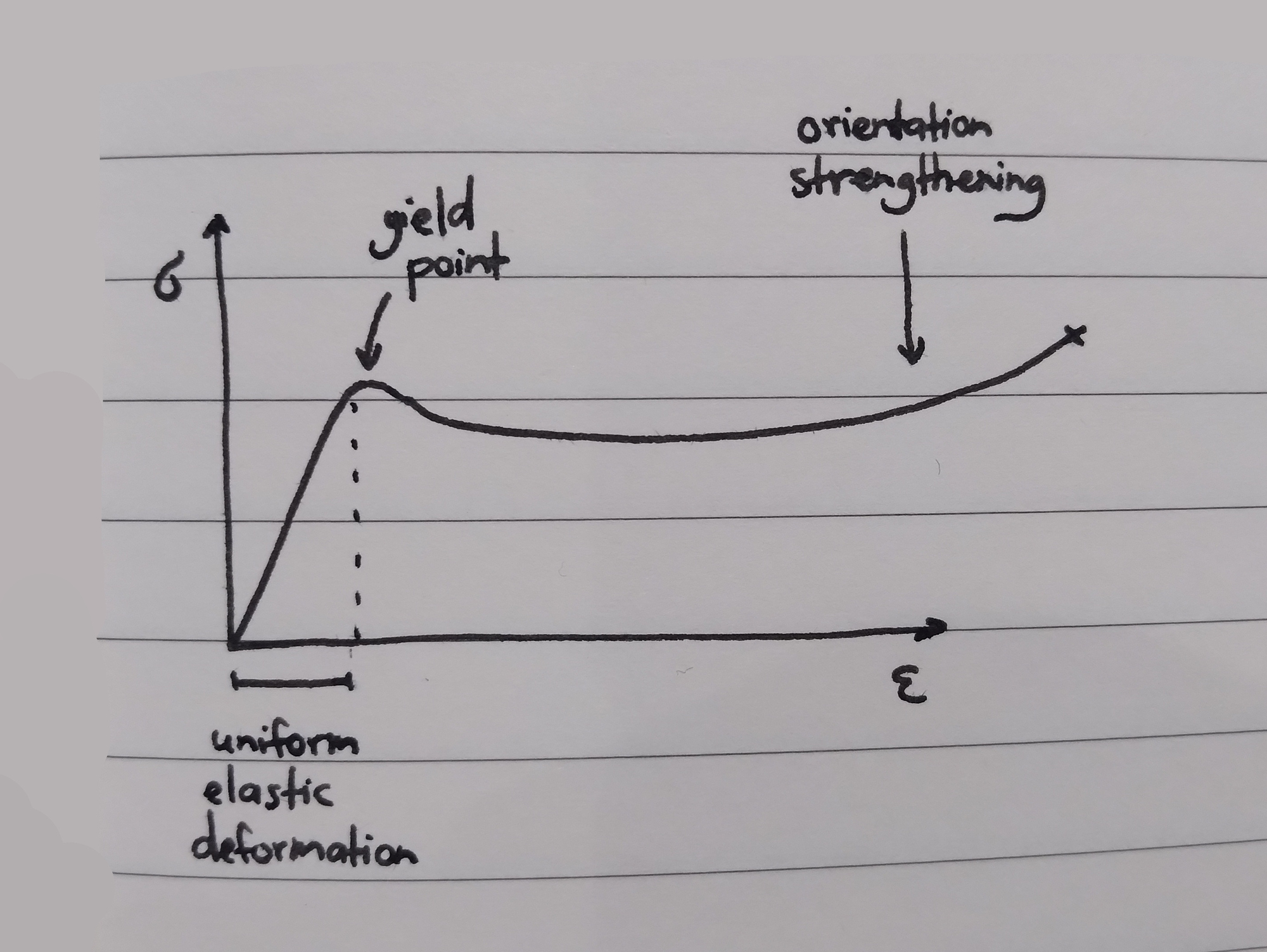
In amorphous polymers above T_g, applied strain causes the polymer chains in the strained region to stretch out and align, increasing the density of secondary bonds (and the degree of crystallinity). These stretched regions now have a higher yield strength than the neighbouring amorphous regions (orientation strengthening), so they will resist further strain. Because of the increased degree of crystallinity, these stretched regions will also be more opaque.
After the yield point in the stress-strain graph, a neck begins to form in the specimen. This neck is a localised reduction in cross-sectional area, but it only reduces so far before orientation strengthening prevents further deformation and the still-amorphous material above and below it begins to stretch instead. This ‘travelling neck’ becomes longer and longer until all available material has been orientation-strengthened and the sample fractures.
In contrast, when a neck forms in a strained metal sample, all subsequent deformation is concentrated in the neck region (the point with the lowest cross-sectional area).
The strength and stiffness of an orientation-strengthened material increases along the direction of the chains (because stress is being opposed by strong covalent bonds), but decreases in the perpendicular direction (because stress is being opposed by weak intermolecular bonds). This results in anisotropic mechanical properties. Cracks can more easily propagate by sliding between the chains.
The deformation of thermoplastic materials can be elastic, plastic, or a combination of both. Elastic deformation occurs below the T_g, plastic deformation above the T_g.
There are three different deformation mechanisms:
Stretching of bonds within each chain (elastic deformation).
Uncoiling and stretching of polymer chains (either elastic or plastic depending if they recoil once unloaded)
Breaking and reforming secondary bonds by sliding chains past each other (plastic deformation)
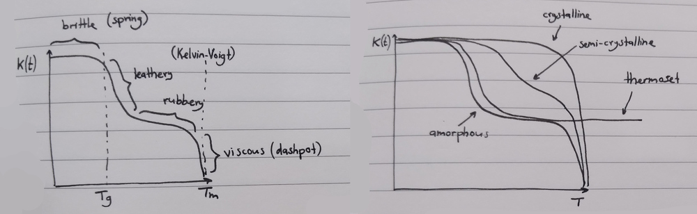
Polymers above T_g can exhibit either elastic or viscous (plastic) behaviour when a constant stress is applied, depending on the magnitude of that stress. Elastic behaviour is modelled as a spring element, and viscous behaviour is modelled as a dashpot element. A combination of behaviours can be modelled with either the Maxwell or the Kelvin-Voigt models:
For a spring element, strain is directly proportional to stress (\sigma = E \x \epsilon). Elastic deformation is instantaneous on loading and recovery is instantaneous on unloading.
For a dashpot element, the rate of change of strain (the gradient of the strain-time curve) is directly proportional to applied stress. Strain slowly increases under constant stress due to chain untangling and sliding, and is not recovered on unloading.
The Maxwell model combines a spring element and a dashpot element in series. When a constant stress is applied, strain instantly increases due to the instantaneous elastic deformation of the spring element, and the dashpot element slowly extends until the strain in the spring is completely restored. On the strain-time graph, this looks like a sudden increase, a linear increase, and then a sudden decrease to a point above zero.
The Kelvin-Voigt model combines a spring element and a dashpot in parallel, with both elements constrained to move together. The strain-time graph looks like that of a resistor-capacitor circuit, increasing rapidly and gradually slower up to a maximum point (due to maximum extension of the spring), and then decreasing rapidly and gradually slower back to zero when unloaded.
The viscoelastic behaviour of polymeric materials depends on time and temperature. We’re given the example of an engine drive-belt in a car that goes slack over time, or a nylon guitar string that needs regular tuning to stay taut. Stress relaxation describes this phenomenon, where a material is under constant strain but where the stress required to maintain this strain decreases over time.
When a constant strain is applied to the Maxwell model, the spring element instantly takes up the full strain, but over time the dashpot element will take up some of the strain from the spring (in decreasing amounts over time). The stress of the whole model reduces in a resistor-capacitor manner as the dashpot takes up all of the strain, decreasing rapidly and then gradually slowing until reaching zero stress. The stress \sigma_t at any time under a constant strain can be calculated from the initial stress \sigma_o, the time t, and the relaxation time constant \tau (in seconds):
\sigma_t = \sigma_o \x \exp(-\frac{t}{\tau})
The relaxation time constant \tau can be calculated from the dashpot viscosity \eta and the spring modulus E:
\tau = \frac{\eta}{E}
\tau is a property of a given material, and can be calculated with an Arrhenius-like equation using a constant C, the activation energy of the polymer Q (\u{J}\u{mol}^{-1}), the universal gas constant R (8.314\u{J}\u{mol}^{-1}\u{K}^{-1}), and the temperature T (\u{K}):
\1{\tau} = c \x \exp(-\frac{Q}{RT})
Under the Kelvin-Voigt model, a constant strain corresponds to a constant stress (that of the spring element), so it cannot be used to model stress relaxation.
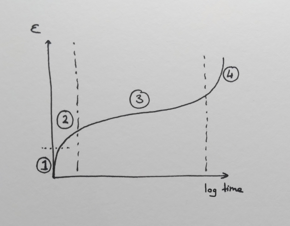
Creep describes the phenomenon where a constant stress is applied to a material and the strain increases over time, gradually slowing to a point. This can be modelled using the Kelvin-Voigt model. The example given to us is a sagging clothesline or bookshelf.
In contrast, a typical metal would undergo instantaneous elastic deformation and then hold indefinitely (this is the behaviour exhibited by a thermoplastic below T_g).
In a thermoplastic above T_g, the polymer chains will slide past each other as long as a stress is applied (as per the Maxwell and Kelvin-Voight models). This means that the strain of the material is time-dependent, and therefore the stiffness / modulus of the material is also time-dependent. We call the time-dependent modulus K(t), giving the modulus at a time t (10 seconds by convention).
K(t) = \frac{\sigma}{\epsilon(t)}
These characteristic responses are due to time and temperature dependent changes in the polymer microstructure.
Linear polymers are formed from repeating monomer units arranged end-to-end with no branching. Chains are long and flexible, and the material can be high density / close-packed.
Branched polymers are formed from a main backbone with attached side branches. Branches prevent the chain from packing close, so the material is lower density.
Cross-linked polymers are formed when polymer chains are bonded together with short covalently-bonded segments, forming a strong mesh.
Thermoplastics (thermoplastic polymers) Thermoplastics are polymers that soften with increasing temperature. They have either linear or branched structures, with weak secondary bonds. These secondary bonds are further weakened by the vibrations caused by heat, but will be restored once the material has cooled. This allows for the material to be reshaped repeatedly.
Thermosets (thermosetting polymers) Thermosets are polymers that do not soften with heat. These are cross-linked polymers with strong covalent bonds. They are hard, strong, and insulating, they char instead of burning, and they can’t be recycled.
Elastomers (includes rubber) Elastomers are polymers that can experience very large elastic deformations. These are formed from highly coiled polymer chains with a few covalently-bonded cross-links to prevent the chains from sliding (which would cause plastic deformation). There’s an optimal number of cross-links, too many links make for a hard rubber and too few links make for a weak and ductile rubber. Elastomers undergo large and non-linear elastic strain in response to stress (unlike metals, which undergo small, linear elastic strain).
Also known as polyethene. Comes in two different forms:
low-density (LDPE, recycling code 4), used for packing foam, bubble wrap, cling film, and plastic bags.
high-density (HDPE, recycling code 2), used for rope, corrugated and flexible piping, and milk bottles.
LDPE has branched polymer structures, preventing tight packing of polymer chains and causing the material to have a low degree of crystallinity (transparent, weak). In comparison, HDPE can pack very tightly.
Also known as Perspex or acrylic. Not recyclable. Used for aircraft windscreens and safety glasses.
The ester side group is very large and prevents the formation of crystallites. PMMA is always completely amorphous (transparent, low density, low strength).
Corrosion is the deterioration of a material resulting from a chemical attack by the environment. Corrosion of metals is an electrochemical process (involving both the movement of electrons and a change in chemical composition).
When \ce{NaCl} is added to water, the \ce{Na} and \ce{Cl} atoms separate (‘dissociate’) into an \ce{Na^+} cation and a \ce{Cl^-} anion. Cations are positive, anions are negative. The resultant solution is called an electrolyte (solution containing dissolved ions). Corrosion can only happen in the presence of an electrolyte.
\ce{NaCl} dissolves in water because it is a ceramic (has ionic and covalent bonds). Metals don’t have ionic bonds, so they don’t dissolve when added to water. Instead, the solid metal atoms transform into ions via an oxidation-reduction reaction (a redox reaction). For example, zinc in dilute hydrochloric acid becomes zinc chloride and hydrogen gas:
This reaction is actually two separate reactions happening simultaneously: an oxidation or anodic reaction (which produces electrons) and a reduction or cathodic reaction (which consumes them). These two reactions much occur at the same time and at the same rate.
\ce{ Zn_{(s)} -> Zn^2+_{(aq)} + 2e^- }
\ce{ 2H^+_{(aq)} + 2e^- -> H2_{(g)} }
The oxidation reaction is the reaction by which metals form cations (positively-charged particles) that dissolve into an aqueous solution. This generates electrons and makes the metal corrode (lose mass). It’s also called an anodic reaction because it takes place on the anode (negatively-charged terminal). Electrons produced by the reaction join the ‘sea of electrons’ inside the metal, to be consumed by the reduction reaction.
The reduction reaction is the reaction by which cations accept the spare electrons generated by the oxidation reaction. It’s also called a cathodic reaction because it takes place on the cathode (positively-charged terminal). Unlike the oxidation reaction, which only has one form, there are multiple possible reduction reactions which could take place depending on the aqueous environment. Specifically, there are three possible reactions that could occur if the aqueous solution does not contain metal ions:
Water contains dissolved \ce{O2} oxygen molecules from the atmosphere. When a droplet of water sits on a block of iron, we get the following oxidation reaction at microscopic local anodes or the surface of the iron block, where the \ce{Fe^2+_{(aq)}} ions dissolve into the water and the electrons stay inside the iron:
\ce{ Fe_{(s)} -> Fe^2+_{(aq)} + 2e^- }
The surplus electrons generated by the oxidation reaction now react with the water and the \ce{O2} oxygen molecules at microscopic local cathodes on the surface of the iron block to form \ce{OH^-} hydroxides dissolved in the water:
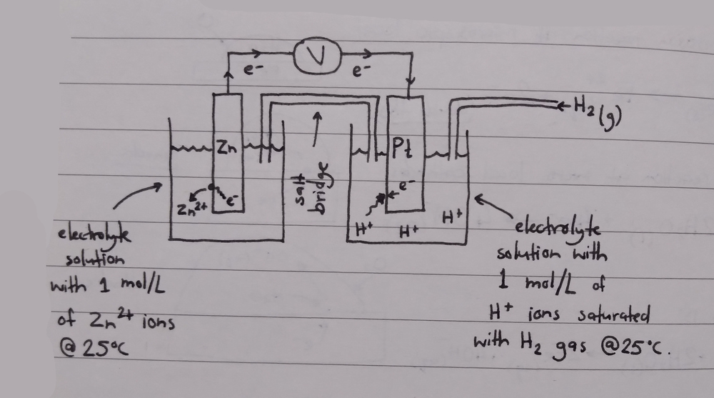
Every metal has a different tendency to corrode in different environments. One method to compare the tendency for a metal to form ions in an aqueous solution (in other words, corrode) is to compare their half-cell oxidation or reduction potentials to a known reference (the ‘standard hydrogen reference electrode’, which we assign the zero voltage).
For this setup, we immerse an electrode of the metal in question in one flask of electrolyte, we immerse an electrode of our reference metal (platinum) in a separate flask of electrolyte, we connect both flasks with a salt bridge to allow the transfer of ions between electrolytes (this has something to do with making the electrolyte solutions electrically neutral), we pump hydrogen gas into the reference electrolyte to create dissolved hydrogen ions, and finally we connect both electrodes with a voltmeter. The voltmeter allows us to see the magnitude and direction of the potential difference, which is related to electron flow.
In this example, zinc atoms undergo an oxidisation reaction to become dissolved \ce{Zn^2+} ions and free electrons, these electrons travel through the voltmeter to the platinum, and the electrons on the surface of the platinum react with the \ce{H^+} ions in the electrolyte to become hydrogen gas.
If the electrode with the higher potential is placed in an electrolyte containing metal ions, the reaction will run in reverse, depositing metallic atoms on the surface of the cathode. The anode strips electrons from hydrogen gas to make \ce{H^+} ions, and these electrons travel to the cathode to react with the \ce{M^+} ions, creating metallic atoms evenly across the surface of the electrode.
When electroplating with the standard hydrogen electrode, the hydrogen electrode must be the anode and the cathode must have a positive potential relative to hydrogen gas.
As per the definition of voltage, the electropotential of the whole cell is equal to the difference between the electropotentials of the reducing electrode (cathode) and the oxidising electrode (anode):
E_\t{cell} = E_\t{reduction} - E_\t{oxidation}
A negative half-cell potential represents the movement of electrons from the unknown electrode to the reference electrode (because voltage polarity is opposite to current polarity), meaning that the electrode is more reactive than hydrogen gas. A positive half-cell potential represents movement from the reference electrode to the unknown electrode, meaning that the electrode is less reactive than hydrogen gas. We need to always remember to say that the half-cell potential is relative to the standard hydrogen electrode.
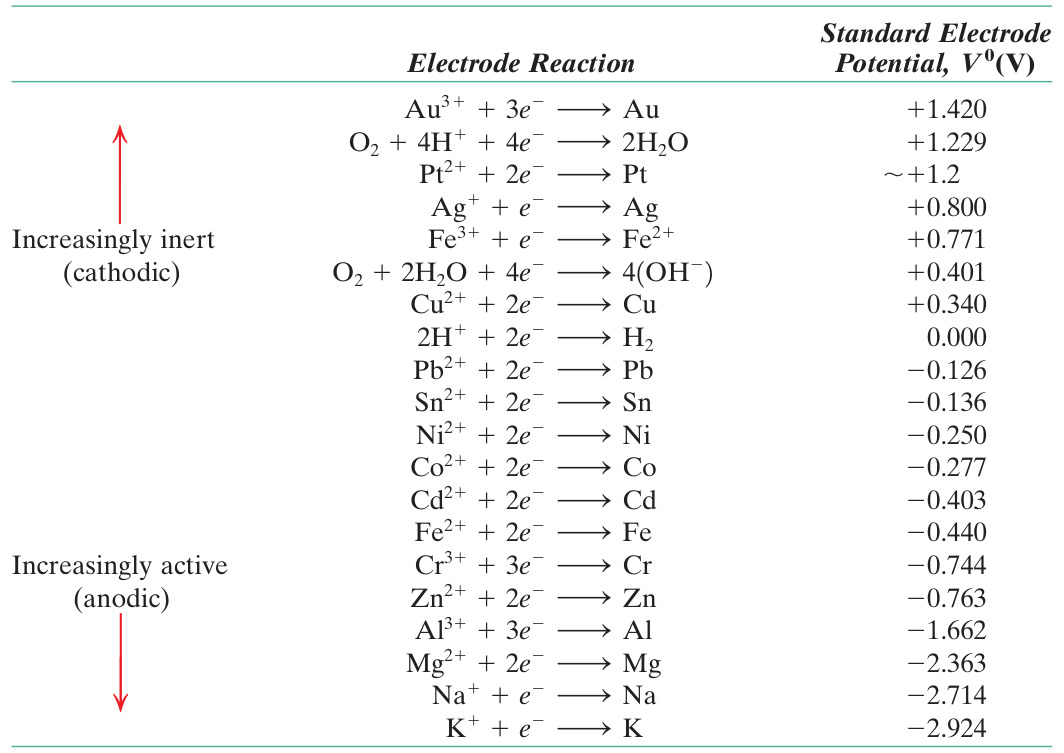
The reaction with the more negative electropotential is the anodic reaction (oxidation, gaining electrons), and the reaction with the more positive electropotential is the cathodic reaction (reduction, losing electrons). The following table shows relative potentials for the reduction reaction (‘standard electrode potentials’), where metals with a lower potential are more reactive / corrode easier than those above.
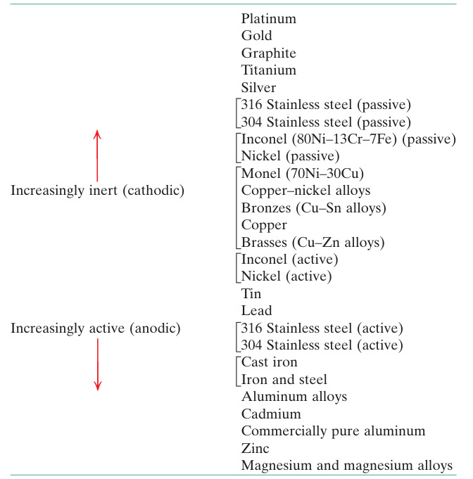
For practical applications (outside a laboratory, without access to a platinum electrode and hydrogen gas), we can use a galvanic series, a table that ranks metals as more or less reactive in a given corrosive environment. The following table is for metals in flowing seawater. Metals listed as passive have a protective oxide layer, metals listed as active do not.
Most metallic corrosion involves an electrochemical reaction that can be modelled as a galvanic cell. A galvanic cell has four components — remove any one component and corrosion will cease:
An anode, which undergoes corrosion to provide electrons to the circuit.
A cathode, which receives electrons from the circuit. The reduction reaction creates a by-product at the cathode.
An electrical connection to permit the flow of electrons from the anode to the cathode.
A liquid electrolyte that is in contact with both anode and cathode and is electrically conducting (contains impurities) to allow electrons to move from the cathode back to the anode.
A composition cell is formed from two dissimilar metals immersed in an electrolyte. The metal which is lower on the galvanic series is the anode (will corrode), and the metal which is higher is the cathode (will not corrode).
We’re given the example of a galvanised steel plate with a scratch on it, with a droplet of rainwater sitting over the scratch. The rainwater is the electrolyte, the surface coating of zinc is the anode (lower on the galvanic series), and the exposed iron is the cathode. The anodic (oxidising) reaction will be the corrosion of the zinc via \ce{Zn_{(s)} -> Zn^2+_{(s)} + 2e^-}, and the cathodic (reducing) reaction will be the production of hydroxides via \ce{O2_({g}) + 2H2O_{(l)} + 4e^- -> 4OH^-_{(aq)}}. This is sacrificial anodic protection.
The electroplating reduction reaction can’t happen at the iron because of the lack of \ce{Fe^2+} iron ions in the rainwater.
Another example is with tin-plated steel cans used for food storage. In this case, tin is cathodic and steel is anodic, and so if the tin is scratched the steel will corrode. This is bad, because the steel will eventually fail with enough corrosion, but the reason tin is used is because it’s non-toxic compared to zinc, and because in the oxygen-low environment of the can the tin is actually anodic to steel.
Composition cells can be created when two pipes of dissimilar metals are joined directly — the metals form the anode and cathode, the direct connection creates a physical electrical connection, and the water flowing through the pipe is the electrolyte. This will cause the pipes to corrode aggressively. The galvanic cell can be broken by using an insulating plastic pipe joiner.
Dissimilarity of metals creates a tendency for metals to corrode, but the actual rate of corrosion is determined from the relative difference in surface areas between the anode and cathode.
If the anode is small relative to the cathode, it will corrode very fast. If the anode is large relative to the cathode, the anode will corrode very slowly. This is because a reduction reaction of equal magnitude must occur simultaneously to the oxidation reaction, and the speed of the reduction reaction is limited by the number of oxygen atoms in contact with the surface of the cathode (which is proportional to surface area). In contrast, the oxidation reaction will always have a ready supply of metal atoms in contact with electrolyte, so the conversion of metal atoms into metal ions can happen as fast as needed.
During galvanic corrosion, electrons flow from the anode to the cathode (creating a current). For a given current flow, more electrons are stripped from the anode per unit surface area for a small anode than for a large anode. The amount of current flowing per unit surface area in the anode is called the current densityi (\t{A}\u{m}^-2), and is given by the total current I (\t{A}) and the anodic surface area A (\t{m}^2):
i = \frac{I}{A}
One example is steel plates connected together with aluminium bolts. Aluminium is the anode (lower on the galvanic series), steel is the cathode, and the bolt is much smaller than the plate, so the bolt will corrode rapidly. If steel bolts and aluminium plates are used instead, corrosion will be very slow.
The amount of metal m (\t{g}) removed from the anode by corrosion can be determined by Faraday’s equation, using the galvanic current I (\t{A}), time t (\t{s}), atomic mass of the metal M (\t{g}\u{mol}^{-1}), number of electrons exchanged in the anodic reaction n, and the constant Faraday’s number F (96,500\u{C}\u{mol}^{-1}):
m = \frac{I \x t \x M}{n \x F}
If the oxidation reaction is \ce{Fe -> Fe^2+ + 2e^-}, then n will be equal to 2 (the number of electrons generated by the reaction).
A composition cell is formed from a single type of metal submerged in an electrolyte with a concentration gradient. The metal in contact with the more concentrated solution is the cathode, and the metal in contact with the more dilute solution is the anode. We’re only going to look at the oxygen concentration cell.
The experimental setup has two electrodes within a single flask of electrolyte with a membrane separating both sides, a physical electrical connection placed across the electrodes, and oxygen gas bubbled into the electrolyte on one side.
There are six examples we’re given for oxygen concentration cells in real life:
Crevice corrosion Occurs when two steel plates are bolted together with steel bolts. No matter how tightly the plates are joined, there will always be a narrow gap (or crevice) between the plates. When the steel is wetted by rain, oxygen in the atmosphere can dissolve into the water. The oxygen is more likely to reach the surface of the steel outside the crevice than the steel deep inside the crevice (because the distance between the surface of the water and the surface of the steel is shorter outside the crevice), creating an oxygen concentration gradient that turns the inside of the crevice into an anode and the outside into a cathode. Crevice corrosion can be mitigated by using a metal washer, or (even better), a plastic washer to fill the gap.
Droplet corrosion When droplets of water sit on a metal surface, the distance between the water surface and the metal surface is larger in the center of the droplet than at the edges of the droplet, which means that oxygen can more easily reach the metal at the edges of the droplet. This forms an oxygen concentration gradient, leading to corrosion of the metal at the center of the droplet.
Pitting corrosion Once a small amount of metal is eaten away by another form of corrosion, a ‘pit’ forms in the material. The distance from the water surface and the bottom of the pit will now be even greater than before, leading to even faster corrosion as the pit grows deeper.
Water-line corrosion When water is stored in a metal tank, a meniscus forms at the interface between the tank wall and the surface of the water. This creates an oxygen concentration in the same manner as for droplet corrosion. Water-line corrosion can be mitigated by constantly changing the amount of water stored in the tank, moving the water line.
Buried steel corrosion When metal is partly buried in damp soil, oxygen will be able to diffuse to just below the surface of the soil but no further, creating an oxygen concentration gradient. The buried metal will be the anode (oxygen-poor), and the metal at the surface will be the cathode.
Buried pipes When a pipe is buried beneath soil of varying compactness, the pipe beneath the looser soil will contain more oxygen than the more compact soil, with the water moving through the pipe acting as the electrolyte. The pipe segment beneath the denser soil will be the anode (oxygen-poor), and the pipe segment beneath the looser soil will be the cathode.
Proximity is important for the redox reaction to occur. The reaction is more likely to occur where the anode and cathode are close, because it’s more likely for the electrons to complete the journey. If a closer cathode is available, the electrons will travel there instead.
We have a few different methods of protecting against galvanic corrosion.
Remove the electrolyte by designing components with proper drainage so that water can’t sit in or against them for long periods of time, and clean away water-bearing surface deposits from the surface (mud, bits of food).
Remove the anode (cathodic protection) by changing the materials so that the anodic material becomes cathodic, or galvanise the anode / add a sacrificial anode to do the same. The sacrificial anode donates electrons to the metal, forcing it to become a cathode. Another approach is to attach a DC battery directly to the anode, using an inert graphite block as an anodic ground point — this will cause electrons to flow from graphite to battery to metal, forcing the metal to become a cathode.
Remove the cathode by covering it with a protective coating to isolate it from the system. This could be paint (an electrically insulating polymer), or a passivated layer (oxide layers on aluminium or stainless steel), or it could be an electroplated metallic coating (zinc, tin).
Remove the electrical connection between the anode and cathode by using insulating materials between dissimilar materials (plastic washers, or plastic pipe joiners).
Fracture occurs when a crack propagates through a material, forming two new fracture surfaces. These surfaces can only be created through the breaking of intermolecular (covalent) bonds, which requires a large amount of energy. As stress is applied to a cracked material, the crack extends deeper and deeper into the material until it reaches the other side, leading to fracture.
The amount of energy required to fracture a material can be seen as the area underneath the stress-strain curve up to fracture, which is the stress multiplied by the strain. Stress is force per unit area and strain is distance, so this is the same as work done (force times distance), which is energy (given in joules).
There are two main types of fracture, ductile and brittle.
In ductile fracture, the material plastically deforms right up to the point of fracture, so a lot of energy is consumed by the plastic deformation occurring at the tip of the crack. As the crack gets deeper, the crack also gets wider, which consumes even more energy. Materials that undergo ductile fracture are normally very tough.
Energy must be supplied continuously for the crack to propagate (‘stable crack growth’). If stress is removed, the crack stops advancing.
There are three distinct stages in the tensile fracture of a ductile material:
Necking begins when you reach the ultimate tensile stress. A large amount of plastic deformation occurs in the necked region, which results in the formation of micro-voids around microscopic particles (such as oxide inclusions) and grain boundaries.
As plastic deformation continues, the micro-voids begin to coalesce into a large central void (flattish, perpendicular to the tension force). The cross-sectional area is greatly reduced, which massively increases internal stress.
The flat central void propagates out towards the surface, creating an elliptical crack. Final failure occurs along 45° shear planes, creating the characteristic cup-and-cone fracture form (one side of the fracture will exhibit a concave ‘cup’ shape, and the other will exhibit a convex ‘cone’ shape).
Each grain in the material also undergoes microscopic failure through extreme deformation and micro-necking. This means that the fracture surface of a ductile fracture will always be microscopically rough.
In brittle fracture, the material fractures quickly with minimal plastic deformation and without much warning. The crack can’t stretch to become wider because brittle materials are resistant to plastic deformation / dislocation movement, so it gets deeper instead, cleaving through the material. The lack of plastic deformation means that brittle fracture takes less energy than ductile fracture.
Brittle fracture surfaces tend to be flat and featureless, and are due to a crack propagating along crystal planes (cleavage) or along grain boundaries. Fracture surfaces are not deformed, and can fit together neatly.
Pre-existing cracks or flaws in a material can create stress concentrations, where the stress around the crack is exponentially larger than the stress in the uniform portion of the material. We can visualise stress lines as deflecting around the curve, bunching up where there isn’t as much room to navigate.
Brittle fractures tend to occur:
in low temperatures (inhibits dislocation movement)
with sudden loading (not enough time for dislocation movement)
around cracks, sharp notches, and flaws (stress concentration)
in a ductile material where there is a brittle phase near the grain boundaries of a ductile phase (inhibits dislocation movement)
Brittle fracture is unpredictable. If you perform a tensile test on a brittle material ten different times to find the yield strength, you’re likely to get ten different numbers.
Toughness is also difficult to quantify. A ductile material undergoing tensile testing could fracture in a more brittle manner with the presence of notches or other surface defects, so the area underneath the stress-strain curve is only an approximation of toughness.
Toughness can be more reliably measured using the Charpy impact test. A hammer of a known mass is attached to a pivot and dropped/swung from a fixed height through a sample placed at the bottom of the swing. The hammer continues to swing through the arc after the sample has fractured, with the maximum height attained by the hammer after this point being used to determine the amount of energy that was lost to the impact. A tougher material will absorb more of the hammer’s energy, and a more brittle material will absorb less. We call the initial height of the hammer from the ground h_0 (when the hammer is parallel to the ground), the final height of the hammer h_f, and the difference \Delta h = h_0 - h_f is proportional to the amount of energy used to fracture the sample.
To compare the toughness of two different materials, we need to have specimens with identical dimensions and identical notch geometry. This notch creates an area of high stress concentration. Notches make a material more susceptible to brittle failure even if it would otherwise be quite ductile if there was no notch present.
Notches create sites of high stress concentration, where a material is most vulnerable to brittle fracture (less ductile than it otherwise would be).
This can be seen by drawing tensile force contours. The notch creates a narrow region where tensile stress is concentrated, meaning that the notched region will yield first. The axial tensile stress experienced by the material at the tip of the notch is huge, but gets smaller the further you move from the notch in either direction. The proximity of high stress concentrations and low stress concentrations creates a shear stress.
A fracture at the notch will be accompanied by a transverse Poisson contraction, but this contraction is resisted by the surrounding less-stressed material. This generates secondary tensile stresses in the transverse direction acting in opposition to the contraction. This means that in order for plastic deformation to occur in the axial direction, a higher stress must be applied to overcome the secondary tensile stresses, with this higher yield stress making the material more brittle (by definition). The combination of an axial tensile stress and secondary transverse tensile stress at the notch root is call a state of triaxial stress.
BCC metals are brittle at low temperatures but ductile (and therefore tough) above a certain ductile-brittle transition temperature T_t.
The brittleness of BCC metals is due to the lack of slip systems in the BCC crystal lattice (as opposed to the close-packed FCC lattice), making it difficult for dislocations to move in most directions. As the temperature of a BCC metal increases, atoms move around more due to thermal vibrations, and this movement creates more slip systems where they didn’t exist before. In contrast, freezing a BCC metal will reduce the number of effective slip systems and make the material more brittle (reducing the toughness). The transition is quite sudden, not gradual.
We want to keep the temperature of our metals above T_t when working with them. T_t is influenced by:
Composition Alloying elements increase the ductility of a material, decreasing T_t. Low-carbon steel is hypo-eutectoid / contains more ferrite, which has a ductile BCC lattice structure (compared to cementite, the other phase).
Impurities Iron oxides and iron sulphides will stop dislocation movements in steel, increasing brittleness and increasing T_t. Manganese bonds with sulphur (because it’s more reactive than iron), so adding manganese to steel will reduce sulphide impurities and decrease T_t (around 1-2% manganese is used).
Grain size Cracks form more easily around grain boundaries. Large grains will have large grain boundaries and will encourage the development of large cracks, increasing the brittleness of the material and increasing T_t. This overrides the logic of Hall-Petch, where smaller grains make a material more brittle by blocking dislocations.
Loading time Dislocations take time to move, so there’s less time for dislocations to move when loads are applied quickly, increasing the brittleness of the material and increasing T_t.
Crack geometry Sharp corners create stress concentrations, increasing the brittleness of the material and increasing T_t.
An edge crack is a notch in the edge of a surface, and is characterised by the depth a of the crack into the surface. An internal through crack is a crack that passes right through a material between two faces, and is characterised by the length 2a of the crack across one face (a measures half the length of the crack from point to point).
The stress concentration at the tip of a crack is described by the stress intensity factor K_1, which is given by the applied stress \sigma (\t{Pa}), characteristic crack size a (\t{m}), and a constant geometric factor Y:
K_1 = Y \x \sigma \x \sqrt{\pi a}
When K_1 reaches or exceeds the critical value K_{1c} (the ‘critical stress intensity factor’, or ‘fracture toughness’), the crack will propagate through the material at the speed of sound, causing brittle fracture. The value of K_{1c} depends on the material, with a higher K_{1c} indicating a material of higher ductility / higher toughness.
Cracks can be tolerated in a material so long as K_1 does not reach the K_{1c} for that material.
Fatigue failure occurs when a crack grows slowly over time. This can happen even when the stress is lower than the value required for fast fracture (as above). Fatigue failure is responsible for more than 90% of metallic failures, and can cause failure below the yield stress of a material and brittle fracture in ductile materials. Risk factors are corrosive environments and cyclic stress patterns (‘fatigue loading’).
Examples of situations where fatigue failure can occur are bridges (variable vehicle loads), aircraft and street lights (variable wind loading), water pumps, gear teeth, and pressure vessels (variable fluid loads).
For fatigue failure to occur:
There must be a cyclic stress with a tensile component, which causes cracks to open up and advance. Extremely brittle materials (stones) can be used to build bridges as long as the material is always in compression.
The maximum cyclic stress \sigma_\t{max} must be lower than the yield stress \sigma_{y} of the material, otherwise plastic deformation will occur and the material will fail by a different mechanism.
There must already be a crack (due to corrosion, surface imperfections, or grain boundaries) that can grow to the point that the cross-sectional area of the remaining unfatigued material cannot bear the applied load. This size is calculated using the stress intensity factor.
Fatigue can occur over fewer cycles when the peak stress \sigma_\t{max} is higher.
Fatigue failure can be characterised by the engineering fatigue curve, where the applied peak tensile stress \sigma_\t{max} is graphed against the number of stress cycles experienced by the material.
The fatigue limit / endurance limit of a material is the stress level below which fatigue won’t occur. Ferrous metals have a definite fatigue limit, which is around a quarter to a half of the tensile strength of the material (this definite fatigue limit is caused by work hardening). Non-ferrous metals do not have a definite fatigue limit; instead, their fatigue strength is defined as the number of cycles N that can be achieved before failure occurs (this is normally defined to be N = 10^8).
The fracture surface created by fatigue fracture will exhibit ‘beach lines’ radiating out from the crack initiation site. These beach lines mark major crack advancements. In between these beach lines will be microscopic ‘fatigue striations’, which mark crack advancements at each cycle. Once K_1 /ge K_{1c}, a fast fracture region will be created where the crack instantly propagates the rest of the way through the material. This fracture surface will be heavily textured compared to the smooth striated surface of the fatigued surface.
If the cyclic loading has a compressive component, the crack will open and close repeatedly, rubbing both fracture surfaces against one another and polishing away the beach lines.
Improve surface finish Fatigue can only act on existing cracks and defects. Polishing the surface of a material to remove scratches (stress concentrators) will reduce the tendency for fatigue to occur.
Put surface layer into compression Fatigue can only happen under tensile loads, and higher peak tensile stress increases the tendency for fatigue to occur. By shifting the stress-time graph downwards, the peak tensile stress is reduced without affecting the actual stress range. This can be done through shot peening, where tiny stainless steel balls are blasted at a surface to compress it. Tempering can be used to add residual compression to glass (but not metals because of a lack of covalent bonds).
Minimise stress concentrators This will reduce peak tensile stress.
Creep in polymers is a plastic deformation (increasing strain) that occurs over time due to a constant applied stress above T_g. Creep can also happen in metals at high temperatures.
At room temperature, elastic and plastic deformations depend only on applied stress (time-independent / instantaneous deformation, or low temperature deformation). As the temperature increases, a stress which would otherwise only cause elastic deformation will begin to cause a slow plastic deformation (‘creep’). Creep deformation is dependent on stress, temperature, and time.
Plastic deformation is caused by dislocation movement. This is normally due to a high applied force, but it can also be caused by solid-state diffusion (as with annealing), which occurs much faster at higher temperatures. A material approximately begins to creep when the surface temperature is above 30-40% of T_m in Kelvin for metals, or 40-50% of T_m in Kelvin for ceramics (diffusion is more difficult in ceramics due to the covalent and ionic bonds). For iron, T_m is 1809°K, so room temperature is only 16% of T_m. For lead, however, T_m is 600°K, so room temperature is 49% of T_m. This means that lead is vulnerable to creep at room temperature.
Creep usually occurs under constant stress below the yield stress of the material, at temperatures above T_g for polymers or above 30% of T_m in K for metals. The typical creep-time curve for metals, polymers, and ceramics under constant stress has four distinct regions:
1. Instantaneous elastic deformation Caused when atomic bonds are stretched. Small strain, short period of time, linear elastic deformation. Only happens at low temperatures. Don’t worry about it.
2. Primary non-linear creep Small strain, short period of time. Don’t worry about it.
3. Secondary steady-state creep Large strain, long period of time (on the order of thousands of hours), effectively linear plastic deformation (at least when graphed against log time). This is easily controlled, and must be avoided in order to avoid tertiary creep. Called ‘steady-state’ creep. Tends to happen at high service temperatures due to dislocation climb and stress-induced migration of atoms and vacancies. The time at the end of this region is called the creep life of the material.
4. Tertiary creep Large strain, short period of time, fast and uncontrollable. Point of no return, always leads to failure. Must be avoided at all costs, probably by replacing the component before it reaches this point. Happens due to grain boundary sliding, creating micro voids and micro cracks that grow quickly and concentrate stress.
The secondary steady-state creep creep rate \Delta \epsilon / \Delta t (representing the gradient of the creep curve in that section) under constant stress is modelled by an Arrhenius equation, using a creep constant C, activation energy Q (\t{J}\u{mol}^{-1}), gas constant R, and temperature T (\t{K}):
\frac{\Delta \epsilon}{\Delta t} = C \x \exp(\frac{-Q}{RT})
Dislocations are blocked by obstacles (substitutional or interstitial atoms). Vacancies can move through solid-state diffusion to end up replacing/removing the bottom atom of the dislocation plane/edge that is exactly in line with the obstacle, causing the dislocation to rise by one atom into a parallel slip plane, avoiding the obstacle.
This is the main mechanism responsible for secondary creep.
At high temperatures, thermal vibrations increase the number of vacancies in the material, aiding diffusion of atoms under applied stress. Atoms tend to move axially with stress, and vacancies transverse to stress, causing elongation with a reduction in cross-sectional area.
Atoms can diffuse more rapidly at grain boundaries due to the energy associated with strained inter-atomic bonds at grain boundaries. When shear stresses act along grain boundaries, grain can slide relative to one another.
Unlike regular slip systems, grain boundaries aren’t atomically smooth, so the sliding process leaves behind a trail of vacancies that will grow in size to become voids or microscopic cracks. These voids or cracks will continue to grow or join up, increasing the stress on the rest of the structure until creep fracture occurs. The micro-cracks themselves act as stress concentrators, creating triaxial stress conditions that further increase stress.
This process happens very fast, and is the main mechanism responsible for tertiary creep.
Alloy should have a higher melting point Higher melting points correspond with stronger metallic bonds, which slow down solid-state diffusion by increasing the activation energy, reducing the creep rate. This gives a longer ‘creep life’ for the material. We want to aim to keep the ratio T_s / T_m between the service and melting temperatures below 0.3-0.4.
Alloys should have structures that block dislocation movement Examples of structures that block dislocation movements and dislocation climb are ones with solute atoms (matrix distortion), heat-stable precipitates (shouldn’t melt at high temperatures), and secondary phases (grain boundaries).
Try to choose alloys that have strong covalent bonds Covalent bonds are stronger than metallic bonds. Examples are ceramics (such as magnesium oxide) and inter-metallic compounds (such as cementite and theta phases).
Large grain sizes Diffusion is faster at grain boundaries, so larger grains will increase the distance that atoms have to diffuse before they reach a boundary. Mono-crystals are best.
Precipitates at grain boundaries These create brittle and unpredictable materials, but they’ll also pin grain boundaries in place, preventing grain boundary sliding.
Composites combine polymers, ceramics, and metals to create a material with the strengths of the individual components with fewer of the weaknesses. They are anisotropic.
Composites contain two main components:
a dispersed component This is often strong, stiff particles or fibres to improve strength (\sigma_y), stiffness (E), and creep resistance (blocks dislocation movements).
a matrix This is often a polymer or a metal that can transmit stress \sigma to the dispersed component, protect the dispersed component from corrosion/abrasion, and provide toughness (ductile, prevents crack propagation).
Because composite materials are anisotropic, the direction of the applied force affects the properties of the material:
In isostrain, the strain \epsilon applied to the composite parallel to the laminates/fibres is equal to the strain applied to each component.
In isostress, the stress \sigma applied to the composite perpendicular to the laminates/fibres is equal to the stress applied to each component
The modulus of the composite is dependent on the direction of the stress/strain. The modulus in the isostress direction (perpendicular) is lower than the modulus in the isostrain direction (parallel).
Isostrain stiffness E_{C\parallel} (parallel to fibres) is given by the volume fractions V of each component multiplied by the modulus E of that component:
E_{C\parallel} = V_A \x E_A + V_B \x E_B
Isostress stiffness E_{C\perp} (perpendicular to fibres) is given by the same:
The density of the composite \rho_C is calculated simply from the volume fraction V and density \rho of each component:
\rho_C = V_A \x \rho_A + V_B \x \rho_B
The specific modulus of a material \hat{E_C} is the stiffness of the material E_C relative to the weight (given by density \rho_C). This is an important metric in engineering.
Fibre-reinforced composites consist of strong, stiff fibres embedded in a weak, ductile matrix, resulting in optimum stiffness, strength, toughness (dependent on fibre orientation). Modulus is high in isostrain direction, but low in isostress direction. Fibres can be laid out in multiple directions, but this is more expensive and difficult to manufacture. Instead, we can just align the fibres in the direction of stress.
Ideally, fibres are continuous through the length of the material, which can be difficult to achieve in some situations. Discontinuous fibres will still be quite strong as long as they exceed the critical length l_C.
In fibre-reinforced composites, stress is transmitted to fibres due to the shear stresses generated at the matrix-fibre interface. The shear stresses are caused by a relative difference in strain between the matrix and the fibres. The overall stress in the fibre is proportional to this shear stress, multiplied by the length over which the shear stress is acting. The stress in the fibre increases until the fibre strain equals the matrix strain (the isostrain condition).
The stress at either end of the fibre is zero (because the distance over which the stress is acting approaches zero). The slope \theta represents the matrix-fibre bond strength. If the maximum stress \sigma_\t{max} experienced by the fibres is less than the fibre fracture stress \sigma_f, then we aren’t getting the full value out of our fibres, the matrix is supporting too much of the stress.
What we want is for the fibre to take up as much of the stress as possible, such that \sigma_\t{max} = \sigma_f — the length that fulfils this criteria is called the critical length, l_C. When l > l_C, the fibre will fracture and the load will redistribute through the matrix due to isostrain conditions. On the graph, this looks like the peak of the graph being truncated at the \sigma_f line, making \sigma_\t{max} constant in the central region. This means that discontinuous fibres longer than l_C can be treated as continuous fibres.
The force required to pull a fibre out of the matrix is given by the bonded surface area of the fibre (given by the diameter d and bonded length l of the fibre) and the strength of the shear bond \tau. The diameter of the fibre is normally small enough that we can ignore the surface area of the fibre end caps:
To get stronger composites, we can either increase the length l of each fibre in order to increase the surface area that the matrix-fibre bond is acting on, or we can increase the strength of that bond directly.
Small diameter fibres are preferred because:
Given the same volume fraction of fibre in the composite, smaller diameter fibres will give a greater surface area for the matrix-fibre bond to act on.
Smaller diameter ceramic fibres will have smaller pores (imperfections), so will have a higher yield stress.
A rough rule is that fibre-reinforced composites should have a l/d ratio of at least 50 (to ensure that the fibre exceeds the critical length, allowing it to be treated as continuous), so smaller diameter fibres are able to be made shorter while still meeting this rule.
The stress-strain graph of a fibre-reinforced composite in the isostrain condition depends on the characteristics of the ductile matrix and the strong fibre. The stress-strain graph is split into three regions:
Region 1 continues until the yield point of the matrix. The composite experiences elastic deformation (because the fibre and matrix are both elastically deforming), with the modulus being between that of the matrix and fibres.
Region 2 continues until the yield point / fracture point of the fibre (the fibre is brittle). The matrix will plastically deform in this region with the fibres taking up the full stress. The composite response is still linear, but the modulus is lower.
Region 3 continues until failure. Individual fibres in the composite will steadily break, redistributing stress and increasing the strain in bursts. The strain at the beginning of this region is called the critical strain \epsilon_c.
Composite failure is not normally catastrophic because the fibre fragments can hold the ductile matrix together, preventing brittle failure. Not all fibres will break at the same time. Fibre de-bonding and pull-out also takes time and energy, meaning that composites tend to be tough.
Fibre-reinforced composites have greater toughness than either of their individual components. This is because the composite must undergo fibre de-bonding and fibre pull-out in order to fracture. When an isostrain tensile stress is applied to the composite, the matrix will first elastically deform, then a crack will form at the edge and propagate inwards to the fibre, then the fibre will begin to de-bond from the matrix (separating matrix and fibre by ripping the matrix away), and finally the fibre will pull out and fracture.
We’re given the example of a carbon-fibre reinforced polymer (CFRP) with matrix toughness of 5\u{kJ}\u{m}^{-2}, fibre toughness of 0.1\u{kJ}\u{m}^{-2}, and composite toughness of 50\u{kJ}\u{m}^{-2}.
Wood is formed from long cellulose tubes encased in a lignin matrix. These tubes are filled with water when the tree is alive. The water content increases the ductility of the wood, decreasing the strength.
Fibres are normally 3-5 millimetres in length and 28-80 micrometers in diameter, so the length to diameter ratio easily exceeds 50.
Fibres are much finer and denser in ‘latewood’ (summer growth) than in ‘earlywood’ (spring growth). This can be seen visually as rings in the wood. Spring has lots of rain, so larger tubes are needed to transport it all. Summer has lots of heat, so smaller tubes help to prevent evaporative losses.
The dimensions of wood are labelled longitudinal, radial, and tangential.
Wood is weak under compression in the isostress condition because the tubes are hollow, they can be crushed. It’s also weak under tension in this direction (as are all fibre-reinforced composites) because the matrix has to take up the full load itself, the fibres contribute nothing.
Defects:
Knots reduce cross-sectional area under tension, increasing stress, because only fibres can take the load. But under compression, the knot can take the load.
Knots distort grain, changing parallel fibres into perpendicular fibres.
Moisture content:
Given by (wet weight — dry weight) / dry weight.
Green wood can have over 100% moisture content (that is, there is at least as much water as wood). Important to note, compare moisture weight to the dry wood weight.
Wood has free water and bound water in the cellulose tubes. Free water in the center of the tubes evaporates first. When the water bound to the cells starts to evaporate, the wood shrinks, bringing tubes closer together, making the wood stronger.
Drying process:
The free water evaporates completely. The wood strength doesn’t change in this region.
The point at which all free water is evaporated is called the fibre saturation point. The wood typically has a moisture content of around 30% here. The cell walls are fully saturated.
Once the bound water begins to evaporate, the wood begins to shrink. The wood becomes stronger.
Wood is typically dried to a moisture content of 19% or less. The wood doesn’t become any stronger below this point. The wood is green wood above this point, and dry wood below this point. Green timber is susceptible to fungus.